ECONOMICS WORKING PAPER SERIES
TRENDS AND COMPLEXITY OF
USITC FACT-FINDING REPORTS
William
Deese
Darren Sheets
Working Paper 2016-09-C
U.S. INTERNATIONAL TRADE COMMISSION
500 E Street SW
Washington, DC 20436
September 2016
Office of Economics working papers are the result of ongoing professional
research of USITC Staff and are solely meant to represent the opinions and
professional research of individual authors. These papers are not meant to
represent in any way the views of the U.S. International Trade Commission or
any of its individual Commissioners. Working papers are circulated to promote
the active exchange of ideas between USITC Staff and recognized experts outside
the USITC and to promote professional development of Office Staff by encouraging
outside professional critique of staff research.
Trends and Complexity of USITC Fact-Finding Reports
William Deese and Darren Sheets
Office of Economics Working Paper 2016-09-C
September 2016
ABSTRACT
This report explains the context in which fact-finding reports at the USITC are
produced. We assemble data about the types of analyses in the reports and
combine this information with data on the labor needed to produce the reports;
the period studied is 20022014. Based on the
literature about complexity, we develop indicators for organizational and task
complexity and apply these indicators in linear regressions and a stochastic
boosted regression tree model to explain the numbers of hours used to produce
the reports. We find that these indicators explain a significant degree of the
variation in hours per report, which trended upward over the period studied.
Organizational indicators, such as the number of organizational units needed to
produce the report, outperformed the task indicators, which are related to the
approach and types of analyses in the reports.
William Deese
Office of Economics
Darren Sheets
Office of Economics
1. Introduction
The hours required to conduct fact-finding investigations and write reports on trade and competitiveness topics at the U.S. International Trade Commission (USITC or Commission) has trended upward over the past decade. Recent USITC reports tend to be longer than previous reports and frequently incorporate surveys, complex economic models, or other extensive analysis. Acquiring and analyzing information for these reports has frequently required more staff and a greater variety of skills, which makes the organizational structure and the tasks required to produce the reports more complex. For example, “The Commission is challenged in these efforts by the increasing complexity of its investigations, the variable caseload, and resource constraints.”[1]
This study explores the link between the time needed to produce fact-finding reports and the complexity of the organizations and tasks involved in their production. We apply concepts from the complexity literature in the social and management realms. That literature, despite making progress in understanding complexity, presents no standard paradigm for management and social studies and warns that measurement can be difficult and that some subjectivity is unavoidable. We compile data on Commission reports from 2002 to 2014, develop indicators to measure aspects of organizational complexity and task complexity, and link those indicators to the hours required to produce reports.
We find that the number of divisions[2] working on a report and the number of pages of text in the report are the main statistical indicators of organizational complexity, and these indicators explain a large degree of the variation in hours per report. The number of appendices and the presence of a survey are the main indicators of task complexity. The task variables, while important, explain less variation in total hours per report than the indicators of organizational complexity. The statistical analysis employs both linear regression and the recently developed stochastic boosted regression tree model. This latter method permits us to uncover some non-linear relationships, such as the fact that a jump from a low to a medium level of organizational complexity increases the hours per report much more than going from a high to a very high level of organizational complexity.
This paper is organized as follows. First, the background and framework are developed. Next, the database is described, followed by stylized facts. Then we statistically analyze the data and lastly present the conclusions in the final section.
2. Background
This section describes the environment in which reports on topics related to trade or competitiveness are produced. Mostly, the U.S. Congress or the U.S. Trade Representative requests the fact-finding reports in a letter that identifies the topics and objectives of the study and specifies the delivery date. In some instances, trade legislation directs the USITC to carry out studies on certain topics and establishes the time frame, or the USITC undertakes a study on its own initiative.
Temporary organizations, called project teams, produce these reports. Project team members, who are mainly from the USITC’s Office of Operations, have different skills and different supervisors. A project leader directs the work across the different organizational units from the inception (defining the scope and approach and identifying team members) to the final publication of the report. Team members are, at times, assigned to more than one project team, but a project leader or deputy project leader usually leads only one report at a time. The priorities of heads of the different organizational units and team members can differ from those of the project leader. Despite some differences in priorities, project teams almost always complete these reports on time, although rare unforeseen events may result in rescheduling the due dates. Substantial time pressure is common at certain points in the report production cycle.
These reports undergo an extensive internal review by people on the project team and in other offices, including a professional editor, an attorney, and the Commissioners and their staff. Although all reviewers may not be part of the project team, everyone working on the reports charges those work hours to the project.[3]
The complexity of organizing the work of the project teams varies considerably from report to report. Central aspects involve obtaining commitments of suitable personnel to work on the investigation, assuring the development of the desired content, facilitating information flows among team members and other parties, monitoring progress, and reassigning resources as needed. As the size of the team and the number of organizational units involved increases, leading the project team becomes more complex and requires more time.
In addition, coordination with outside groups is frequently required to arrange meetings with industry representatives or to acquire information needed for the report. Most projects incorporate a public hearing, and the reports include the views of hearing participants and those making written submissions. Domestic or foreign travel, at times, is required to obtain information for the reports, and travel must be coordinated with outside parties and mesh with the project’s work schedule.
General tasks by individual team members involve reviewing literature and gathering and analyzing primary information or secondary information from industry experts and other sources. Specialized tasks include assembling the data, developing and running economic models, performing econometric or other statistical analysis, or technical industry analysis. Team members organize information, write their sections or chapters, prepare supporting tables and graphics, and edit and fact-check the report. Other team members physically produce the reports, which are published in-house.
3. Framework
This section looks at the literature on complexity to develop a framework for this study. The relevant literature, although fairly extensive, provides no generally accepted definition of complexity. A key notion in the literature is that complexity involves a large number of components interconnected to different degrees. Increasing variability makes a system more difficult to predict and to control and contributes to its complexity. The number of different components in a system or the number of interactions among the parts similarly contributes to a system’s complexity. Others view a system as being more complex if it contains more information.
We focus on complexity research in management as being the most relevant for this study, and virtually all empirical studies in this area find complexity to be difficult to measure. For example, Zeltzer et al. (2013) state that objectively quantifying complexity is a large challenge and that measuring it will always involve subjective judgment. Xia and Lee (2005) use an extensive survey to evaluate the complexity of information system (IS) projects, including the structural complexity of IS projects and the uncertainty of changing project environments. They find the duration of a project, its organizational complexity, and its technical or IS complexity to be the major determinants of project complexity. Indicators of organizational and IS complexity are based on factors specific to the IS industry.
Related research focuses on the complexity of tasks and organizations. Liu and Li (2012) develop a theoretical model of task complexity but do not test it empirically. In their model, task complexity is decomposed into the following components:
1. the number of actions or steps needed to complete the task
2. the variety of actions
3. the ambiguity of the actions or possibility of misleading information
4. the interdependency between task components
5. mismatches and the heterogeneity of task components
6. cognitive or physical difficulty inherent in the task
7. time pressure and related temporal constraints.
Damanpour (1996) in a general study on organization and innovation proposes two basic measures of organizational complexitystructural complexity and organizational size. Structural complexity is defined as the number of locations where work is performed, the number of jobs or services coordinated, the extent to which an organization is divided into different structural units, and the variety of specialists in the organization. Damanpour believes size to be an important factor because it increases the coordination cost and large organizations may be less flexible in adapting to change, although additional resources available in a large organization may be a benefit in completing a project quickly.
We considered directly measuring the complexity of the language in the reports. Algorithms exist to measure the complexity of text based on vocabulary, syntax, and other features. We do not take this approach because Commission reports are edited, and efforts are made to write simply and to make the reports accessible to the educated general reader even if the underlying material is technical or of an advanced nature. Thus, we do not believe that these algorithms would score reports in a useful way for our purposes.
We combine ideas from the research on tasks and organizations and develop observable indicators related to the complexity of completing frequently performed tasks to produce the reports and organizing the work of the project teams. A study to observe people engaged in different tasks and to measure the complexity of those tasks directly is infeasible. Instead, we construct a dataset based on existing reports and retrospectively create indicators of task and organizational complexity and link those indicators to hours worked on the reports. The next section describes the dataset created for this purpose.
4. Data
The data originate from three primary sources and are merged into a unified dataset. The following subsections describe the three sources.
4.1 Information on investigations
The Commission maintains information on all its trade and competitiveness investigations initiated since 1930. We first extract data on those that started after 2001.[4] This step results in a list of 277 reports.[5] We also extract information on the type of investigation (e.g. reports issued in response to requests under different authorities),[6] initiation and end dates, whether the report is recurring or a single report on a certain topic, etc. One would expect learning to occur in the production of recurring reports so that the tasks to produce them would become more routine, indicating a lower level of complexity than nonrecurring reports.
4.2 Information on labor costs
Next, we retrieve data on labor costs and match them with the previously discussed data about investigations. The labor cost data is the level of an individual staff member who charges his or her work hours to codes that are tied to specific investigations in particular pay periods. We aggregate these data to determine the total hours that all staff spend on a report.[7] Total hours worked on a report becomes the main response variable in this study. We also extract and aggregate data in different ways to determine the number of divisions that worked on a report, the number of staff members that worked more than 39 hours on a report, and the number of hours for those staff that worked more than 39 hours on a report. For this analysis, divisions are only counted if their members spent more than 30 hours on a report. The number of divisions potentially indicates the report’s organizational complexity because the schedules and work of team members with different skills across different organizational units must be coordinated. Similarly, increases in the number of staff with more than 39 hours charged to the report or in the hours that staff charged to the report contribute to the organizational complexity of producing the report.
4.3 The reports
Lastly, we glean information directly from the reports on basic characteristics to obtain indicators of task and organizational complexity. We obtain information on the number of pages in the report,[8] the number of chapters, and the number of appendices (as well as pages in the appendices). The number of pages in a report is an indicator of organizational complexity because large complex studies typically have long reports. Similarly, more chapters indicate that a report covers more topics, which increases its organizational complexity. Reports often include additional appendices to explain economic models and other complex analyses and to present information too technical for the body of the report; thus, the number of appendices is an overall indicator of the technical complexity of tasks involved in producing the report. We obtain information on the number of countries investigated in a report and expected that additional countries would contribute to a report’s complexity.[9] However, the number of countries turned out not to be very informative because many complex studies focus on a single country or on a type of trade instead of on countries. We also obtain information about areas of strategic research and whether the report employs a new approach.[10] Strategic research areas are noted in the Commission’s Annual Performance Plans and include priority areas to enhance capabilities to analyze new issues in trade and industry competitiveness. Thus, the presence of a strategic research area indicates that the tasks used to produce the report are more complex. New approaches are believed to require new skills and are similarly an indication of the complexity of the tasks used to produce the report.
We obtain information about the use of computable general equilibrium (CGE) modeling, partial equilibrium (PE) modeling, surveys, and econometric analysis. Creation of these parts of reports is believed to be cognitively difficult, and thus the presence or absence of these types of analyses indicates the complexity of the individual tasks used to make a report. First, we create variables for different levels of complexity in CGE modeling, surveys, and econometric analysis. After reviewing reports with PE models, we could only distinguish a single level of complexity for them. An expert in CGE modeling scored the reports with CGE models as being at a standard or advanced level of analysis.[11] Surveys can have two levels of complexity. The standard approach uses informal methods, i.e. contact lists, to identify the sample, and the other level uses a full probability-based survey with a formal sample frame, followed by inferential statistical analysis. The Commission began carrying out probability-based surveys around 2010. Lastly, an expert in econometrics scored the econometric analyses into three levelsstandard, moderate, or advanced.[12]
4.4 The combined database
The combined database has 233 observations, about 16 percent fewer observations than in the original data on investigations.[13] The assembly of the unified data is an accomplishment of this research. The data are in a form that could be updated as new projects are completed. Nevertheless, variables that correspond to many aspects of task and organizational complexity as described in the literature review (section 2) could not be identified, and some variables rely on subjective judgment.
Summary statistics for the variables of interest in the unified database are presented in table 1. The variable recurring equals one if the report is recurring and zero otherwise. The variables econometrics, survey, CGE, and PE are all categorical variables as described in the previous section, with the range of allowable values noted in the table. Tables 2 and 3 list the reports with the most and least hours respectively. India Trade Barriers required the most hours of any report, and the report on U.S.-Morocco FTA required the least. The hours devoted to both the shortest reports and the longest reports have both generally trended upwards over time.
Table 1. Summary statistics
|
Variable |
CV* |
Mean |
Stand. Dev |
Min |
Max |
|---|---|---|---|---|---|
|
No. of divisions spending over 30 hours |
0.52 |
7.1 |
3.7 |
1 |
17 |
|
Days |
0.58 |
199 |
115 |
13 |
594 |
|
Appendices |
0.60 |
4.2 |
2.5 |
0 |
15 |
|
Text pages |
0.63 |
169.9 |
106.9 |
12 |
588 |
|
Chapters |
0.65 |
4.9 |
3.2 |
0 |
28 |
|
No. of staff over 39 hours |
0.73 |
17.3 |
12.7 |
1 |
61 |
|
Total hours |
0.92 |
4,458 |
4,096 |
75 |
23,004 |
|
Hours for staff over 39 hours |
0.96 |
4,172 |
4,020 |
43 |
22,446 |
|
Appendix pages |
1.04 |
44.8 |
46.8 |
0 |
450 |
|
Recurring |
1.42 |
0.33 |
0.47 |
0 |
1 |
|
PE |
1.53 |
0.30 |
0.46 |
0 |
1 |
|
Countries |
1.64 |
3.72 |
6.10 |
0 |
48 |
|
CGE |
2.24 |
0.25 |
0.56 |
0 |
2 |
|
Survey |
3.25 |
0.12 |
0.39 |
0 |
2 |
|
Econometrics |
3.79 |
0.14 |
0.53 |
0 |
3 |
Source: Database compiled by USITC staff.
* CV is the coefficient of variation or the standard deviation divided by the
mean.
Table 2. Reports with the most hours, by year
|
Number |
Title |
Year |
Total hours |
Total pages |
Days |
|---|---|---|---|---|---|
|
332-448 |
Textiles and Apparel |
2003 |
22,556 |
583 |
263 |
|
332-460 |
Foundry Products |
2005 |
18,482 |
368 |
335 |
|
332-481 |
Industrial Biotechnology |
2008 |
18,387 |
182 |
583 |
|
332-519 |
Effects of China's IPR |
2011 |
17,894 |
308 |
342 |
|
332-543 |
India Trade Barriers |
2014 |
23,004 |
465 |
476 |
Source: Database compiled by USITC staff.
Table 3. Reports with the least total hours, by years
|
Number |
Title |
Year |
Total hours |
Total pages |
Days |
|---|---|---|---|---|---|
|
103-009 |
Sanitary Articles of Rayon |
2004 |
152 |
22 |
50 |
|
103-011 |
US-Morocco FTA |
2005 |
75 |
28 |
13 |
|
103-013 |
Woven Cotton Boxer Shorts |
2006 |
211 |
26 |
63 |
|
103-018 |
NAFTA Sanitary Articles |
2007 |
162 |
44 |
44 |
|
332-351 |
U.S. Imports of Peppers |
2008 |
155 |
40 |
213 |
Source: Database compiled by USITC staff.
5. Stylized Facts
This section highlights salient trends in the data and should aid in understanding the statistical analysis in the following section. Overall, the hours required to produce the reports have increased along with the indicators of complexity. The trends tend to be gradual, but there are a few abrupt changes.
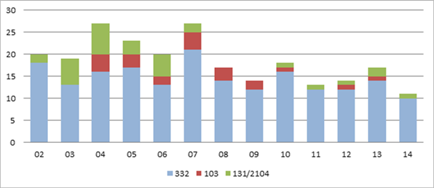
During 20042007, the Commission completed at least 20 reports annually but has not since passed that threshold (figure 1). The number of 103 and 131/ 2104 studies, which are shorter on average, also decreased.[14]
Figure 1. Number of reports completed, by year and type, 20022014
Source: Database compiled by USITC staff.
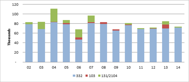
Total hours employed to produce the reports have been fairly stable in recent years (figure 2). The dip in hours in 2011 and 2012 could be associated with voluntary early retirements that were offered during that time.
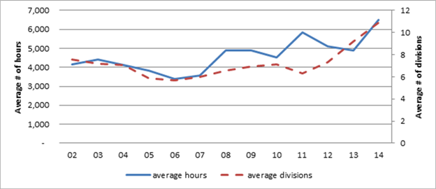
Around 2006, the average number of hours spent on a
completed report and the average number of divisions employed to produce a
report began to rise, although somewhat irregularly (figure 3). The increase in
number of divisions indicates that a wider variety of skills have been used in
the reports and that additional coordination has been needed to complete the
reports, which increases the organizational complexity.
Figure 2.
Total hours for completed reports, 20022014
Source: Database compiled by USITC staff.
Figure 3. Average
hours and divisions for completed reports, 20022014
Source: Database compiled by USITC staff.
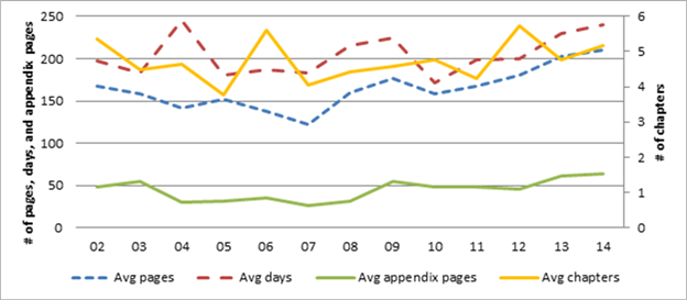
The average number of pages per report after gradually falling since 2002 began
to increase after 2007 (figure 4). The increase from 2007 to 2014 is more than
50 pages per report. During the latter part of this period, the length of the
body of report grew more than that of the appendices, which averaged around 50
pages per report.
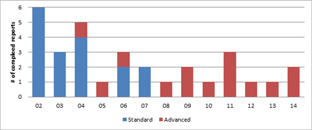
Before 2008, CGE analysis in these reports tended to be at a standard level of difficulty (figure 5). Since 2008, fewer reports have incorporated CGE modeling, but in those that do, the modeling has been more complex.
Figure 4. Trends in report length, 20022014
Source: Data compiled by USITC staff.
Figure 5. Number of
completed reports with standard and advanced CGE analysis, 20022014
Source: Data compiled by USITC staff.
Note: Data about any reports containing classified national security information
have been deleted.
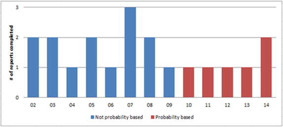
Before 2010, surveys in these reports did not use rigorous statistical techniques to project population-wide results (described as probability sampling in figure 6). However, since then, only probability-based surveys have been used, although the annual number of surveys has decreased.
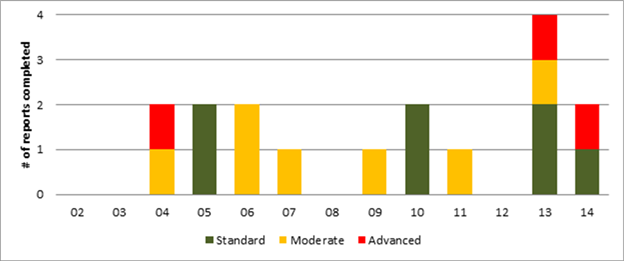
The level of econometric analysis in these reports has not changed greatly throughout this period (figure 7). Nevertheless, the number of econometric studies in these reports jumped to four in 2013, but it is too early to tell if this is a change in trend.
Figure 6. Number of completed reports with different levels of survey analysis, 20022014
Source: Database compiled by USITC staff.
Note: Data about any reports containing classified national security
information have been deleted.
Figure 7. Number of
completed reports with different levels of econometric analysis, 20022014
Source:
Database compiled by USITC staff.
Note: Data about any reports containing classified national security
information have been deleted.
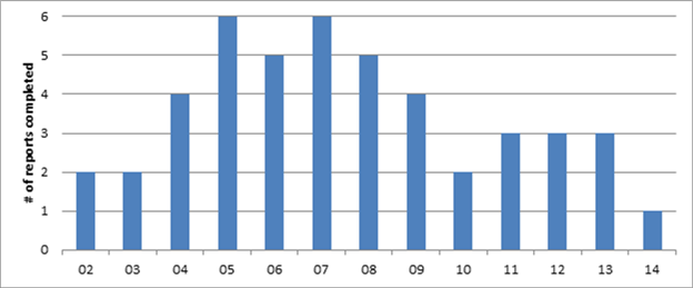
The number of reports with PE analysis was highest in 2005 and 2007 and has
been somewhat irregular in recent years (figure 8).
Figure 8. Number of completed reports with PE analysis, 20022014
Source: Database compiled by USITC staff.
Note: Data about any reports containing classified national security
information have been deleted.
6. Statistical Analysis
In this section, we use two different statistical approaches to examine the effects of the indicators of task and organizational complexity presented in the previous sections on total hours worked per project. Least-squares linear regression, the first approach, is a reliable structured method, in which inference and interpretation are well established, provided certain conditions are met. The other approachstochastic boosted regression trees (SBRTs)is relatively new and appears to be a flexible robust method to uncover relationships between variables, but inference for SBRTs is not well developed, and interpretation mainly relies on graphical results.
As previously discussed, we consider the variables shown in table 4 as indicators of task and organizational complexity. In contrast to the earlier sections, we consolidate most multi-level categorical variables into presence or absence because some combinations have too few observations for reliable statistical analysis. We retain three levels for CGE models. We also include control variables that may influence the number of hours per project.
Table 4. Explanatory variables used in statistical analysis (and levels for categorical variables) by type of complexity and controls
|
Type of Complexity |
Continuous Variables |
Categorical Variables |
|---|---|---|
|
Task complexity |
Appendices
(number) |
Survey (presence
or absence) |
|
Organizational complexity |
Divisions (number
with staff over 30 hours) |
|
|
Controls |
Year |
Type (332, 103, or
131/2104) |
Source: Unified database constructed for this study.
Note: Continuous variables are on the left
6.1 Linear Regression
We transform the response variablehours worked per projectinto natural logarithms, and estimate a log-linear model. The log transformation puts hours worked per project on a scale more similar to other variables and facilitates the interpretation of the coefficients. In this setup, a regression coefficient β for a continuous variable when multiplied by 100 gives the percentage change in total hours per report for an absolute change in the associated explanatory variable, but an adjustment must be made for indicator variables.[15] The semilog equation is shown below where X is a matrix of the explanatory variables with a row for each report; β is a vector of parameters to be estimated, and ε is a vector of mean 0 error terms.
We take several precautions to avoid spurious results.[16] The data span 13 years, and if unavailable variables affect the number of total hours over this period, unobserved heterogeneity could occur and bias the results. For this reason, we include yearly fixed effects.[17] Tests of the residuals show that heteroskedasticity and serial correlation are present; therefore, we estimate robust standard errors that remain consistent in the presence of heteroskedasticity and serial correlation in all runs.[18] Tests indicate that specification is not a problem.[19] Also, we limit the number of variables used because certain combinations of them are exactly collinear. For example, the following equation is an identity in total hours.[20]
One would similarly expect substantial collinearity between text pages, number of chapters, number of appendices, and appendix pages.
The first regression uses a large subset of the available explanatory variables (table 5, column A). This run has a high R2 (0.81), but many variables are not statistically significant, which is characteristic of high collinearity. Still, some continuous variables are significant. For example, the coefficient for divisions indicates that adding an extra division increases the total hours for the report by 14.9 percent. A few categorical variables are also statistically significant. For example, the estimate for 332 reports indicates that this type of report requires around 60 percent more total hours to produce than a section 103 report, which is the base level for comparing report types.[21] This estimate for classified reports shows that they require about 50 percent more hours to complete than unclassified reports.
Table 5. Regression results: Response variable is log of total hours
|
Explanatory variables |
A |
B |
C |
D |
|---|---|---|---|---|
|
Text pages |
0.004*** |
|
0.003*** |
0.003*** |
|
Chapters |
0.016** |
|
0.017** |
|
|
Divisions |
0.149*** |
|
0.147*** |
0.155*** |
|
Appendices |
0.078*** |
0.190*** |
|
0.035* |
|
Appendix pages |
-0.004*** |
0.002* |
|
|
|
Recurring |
0.052 |
0.529 |
|
|
|
Econometrics |
-0.008 |
0.141 |
|
0.029 |
|
Survey |
0.252* |
0.590*** |
|
0.360*** |
|
CGE 1 |
-0.394** |
-0.216 |
|
-0.335** |
|
CGE 2 |
0.076 |
0.553** |
|
0.091 |
|
PE model |
-0.093 |
-0.236* |
|
-0.027 |
|
Strategic research area |
0.234* |
0.465** |
|
0.298*** |
|
New approach |
0.040 |
0.290 |
|
|
|
Classified |
0.394*** |
|
|
0.272*** |
|
332 reports |
0.481** |
|
|
0.574*** |
|
131/2104 reports |
0.279 |
|
|
0.273 |
|
Year fixed effects |
yes |
yes |
yes |
yes |
|
N |
233 |
233 |
233 |
233 |
|
R2 |
0.81 |
0.40 |
0.70 |
0.78 |
Source: Authors’ calculations.
Note: * p < 0.10, **
p < 0.05, ***p < 0.01
The second regression includes the indicators of task complexity (table 5,
column B). Of these, the estimate for number of appendices has the expected
sign and is significant at the 0.01 level. The estimate for survey is also
significant at the 0.01 level and implies that the inclusion of a survey
increases the total hours on a project by around 80 percent. The estimate for
advanced CGE analysis (CGE 2) has the expected sign and is significant, but
standard CGE analysis (CGE 1) is not significant. The estimate for strategic
research areas is significant at the 0.05 level. Estimates for appendix pages,
econometrics, PE model, and new approach are either significant at the 0.10
level or not statistically significant. Also, estimates for recurring reports
are not significant in either column A or column B, implying that there is no
statistical difference in the hours required for these different types of
reports, and we do not examine this variable further. The R2 for this run is only
0.40, which suggests that the task complexity variables by themselves explain
less than half of the variation in total hours, and it is likely that missing
variables may bias the results.
The third regression uses only three continuous explanatory variables linked to organizational complexity but yields a high R2 of approximately 0.70 (table 5, column C). These variables are statistically significant and have the expected positive signs. Reports that are more organizationally complex as indicated by more pages, more chapters, and more divisions require more hours to complete; and the indicators of organizational complexity explain a significant degree of variation in total hours per report.
The fourth regression uses a judicious selection of indicators of organizational and task complexity plus control variables (table 5, column D). Together, these variables explain over 75 percent of the variation in total hours per report (an R2 of 0.78). Indicators of organizational complexitytext pages and divisionsare significant at the 0.01 level and are similar to the estimates in other runs. Given that the average time to complete a report is 4,458 hours, these estimates indicate that adding an extra division increases this time by about 15.5 percent, or by 690 hours, and that an extra page adds 0.3 percent, or 13 hours, to this time. The greater number of hours results not just from the hours that members of a division devote to the project, but also from the increased time that that project leaders and others devote to management and coordination because of the increase in organizational complexity. Similarly, the coefficient on text pages captures the additional coordination and review time and not just the hours required to write an additional page.
Of the indicators for task complexity, the estimate for survey is significant at the 0.01 level, but the number of appendices is only significant at the 0.1 level, both are smaller than the estimates reported in column B, which shows the importance of including the other variables. An additional appendix increases the time required to produce a report by 3.5 percent, or by 156 hours; this variable captures the time devoted to completing various technical tasks and describing the procedure in an appendix. The survey variable is a proxy for the many tasks involved in carrying out a survey, such as designing the questionnaire and the sample frame, obtaining approvals, soliciting the responses, and analyzing the data. The results show that inclusion of a survey increases the total hours for a report by 43.3 percent, or by 1,932 hours. The estimate for strategic research area, a task complexity variable, has the expected sign, and its presence increases the total hours by 35 percent, or 1,548 hours. Estimates for PE model and econometrics, both task complexity variables, are not statistically significant. The estimate for the standard level of CGE analysis (CGE 1) is significant at the 0.05 level but as in the runs reported in columns A and B has a negative sign. Although this suggests that tasks in reports with standard CGE models may be less complex than those in reports without any CGE analysis, the fact that these models are often used in reports that must be quickly completed could mask their underlying complexity. In contrast to the column B run, the estimate for CGE 2 is smaller and no longer statistically significant, although it still has a positive effect on the number of hours per report.
Estimates related to type of report could be characterized as indicating product mix, and their statistical significance underscores their importance. These results show that a 332 report requires approximately 78 percent more hours to complete than a section 103 report. The fact that the Commission completed two or three section 103 reports per year during 20042007 and none or one per year since then explains part of the increase in number of hours per report. The estimate for classified projects indicates that they take approximately 31 percent more hours to complete than non-classified projects.
The column D run includes indicators of organizational complexity and task complexity, as well as controls, and explains much of the variation in total hours, and we view it as the best regression model. We next test the performance of these variables using SBRTs.
6.2 Stochastic Boosted
Regression Trees
Stochastic boosted regression trees (SBRT) have recently received much attention in the statistics and machine learning literatures. Research in biology and medicine frequently employs this method, but there are only a few examples in economics.[22] SBRTs are based on a simple partitioning scheme augmented by modern statistical methods. According to this literature, they produce excellent fits of observed values even when the relationships between the response variable and the explanatory variables are weak (see appendix A for a brief technical introduction). This section presents the results of a SBRT model applied to the project complexity data.[23]
We use the same variables in the SBRT model as in the table 5, column D regression model with two exceptions.[24] First, instead of yearly fixed effects, we include a variable for the year in which a report was completed to capture variation in the time dimension. Second, we initially include the new approach categorical variable. As described more in appendix A, the SBRT algorithm minimizes the deviance (the squared error) between the predicted and observed values of the response variable, and deviance is the primary statistic of interest. Although inference is not well developed for SBRTs, an indication in this case that the fit is good is given by a pseudo R2 of 0.90. SBRT modelers tend to focus more on predictive performance than goodness of fit and split their data into a training dataset and test dataset. They fit the SBRT model to the training data and evaluate its performance with the test data. We apply this approach in comparing the performance of the regression model and the SBRT model in predicting the hours of 2014 projects and find that the SBRT model outperforms the regression model (appendix B).
The SBRT algorithm proceeds in a stage-wise manner and only selects variables that lower the deviance, which usually makes it unnecessary to approximate the significance of individual variables by comparing the deviance of models with and without those variables. In this case, the algorithm initially selects all variables, showing that each of them contributes to lowering the deviance. As is typical in this type of analysis, we evaluate whether to retain marginally selected variables that only have small effects in a backward elimination procedure. Three variables (new approach, econometrics, and strategic research area) only lower the deviance by very small amounts. New approach has virtually no effect, and we prune it out of the model. However, we retain the variables for econometrics and strategic research area because they are important for comparison.
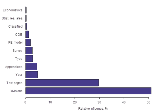
Next, we examine the relative influence of the selected variables in explaining the variation in the number of hours. Two indicators of organizational complexitydivisions and text pages account for, respectively, 51 percent and 30 percent of the relative influence of the selected variables (figure 9). Indicators of task complexity collectively account for slightly more than 11 percent of the relative influence: appendices (5 percent), survey (3 percent), PE model (2 percent), CGE model (1 percent), strategic research area (< 1 percent), and econometrics (<1 percent). Control variables account for slightly more than 8 percent of the relative influence: year (5 percent), project type (3 percent), and classified (< 1 percent). This ranking is largely consistent with the regression column D results. In both cases, divisions and text pages are the main indicators of organizational complexity, and appendices and survey are the main indicators of task complexity. However, the SBRT results show PE modeling to have more influence and CGE modeling to have less influence on numbers of hours per report, compared to the regression results. Also, the inclusion of the variable year makes the importance of the time dimension explicit.
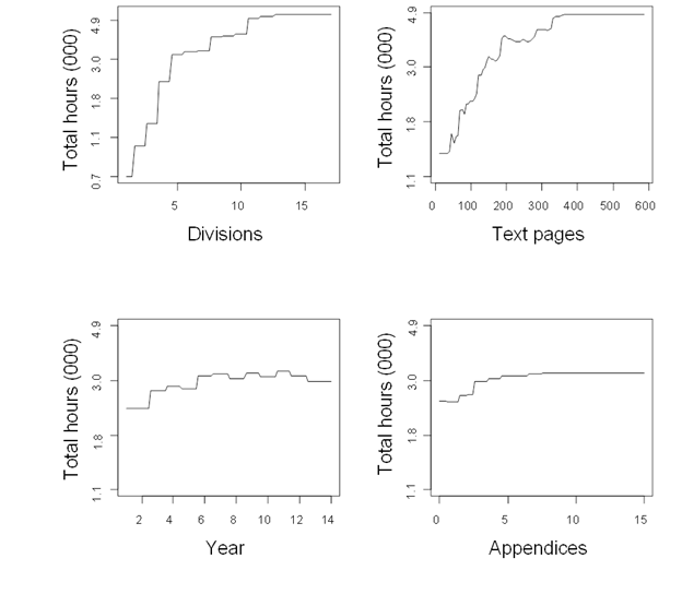
For continuous explanatory variables, SBRTs produce step functions that vary with the response variable, as opposed to the constant slopes associated with regression estimates. Total hours per report increase rapidly as the number of divisions rises from one to five, increase moderately as the number of divisions moves from five to eleven, and remain unchanged with
Figure 9. Relative influence of variables
 Source: Author calculations.
further increases in the number of divisions (figure 10). Fairly similarly,
total hours per report increase rapidly, although irregularly, as the number of
text pages goes from around 50 to 200, rise moderately between 200 and slightly
more than 300 pages, and then are stable. This pattern suggests that going from
a low to a medium level of organizational complexity greatly increases the
hours per report, that going from a medium to a high level of complexity
moderately increases the hours per report, but that going from a high to a very
high level of complexity has little effect on the hours per report. Hours per
report increase moderately as the number of appendices increases from two to
six and then remains constant when more appendices are added. The movement of
this general indicator of task complexity suggests that additional technical
appendices have a small effect on the number of hours per report. The year
variable is associated with fairly small increases in hours up to 2006, then
the effect levels off and falls slightly in 2013 and 2014. The movement of the
control variable year shows that it accounts for some heterogeneity in hours
per report, but its effect is not particularly large because other explanatory
variables now account for the increase in hours per report since 2006 as
reported in figure 3.
Figure 10. Partial influence plots: Continuous variables
Source: Authors' calculations.
Note: To facilitate interpretation, the natural log of total hours (y-axis) is
transformed back to total hours, but the scale remains in logs.
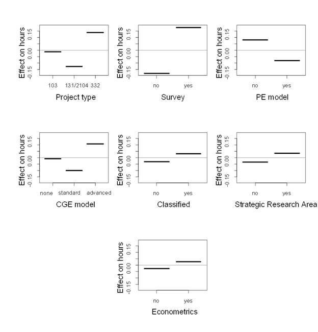
Categorical variables are indicators of task complexity except that project
type and classified are controls. The estimate for survey shows that its
presence adds 43 percent to the hours required to complete a report (figure 11),
which is nearly identical to the regression results (column D, table 5). The
estimates for project type show that 332 reports require approximately 16
percent more hours than a section 103 report, which is qualitatively similar to
Figure 11: Partial influence: Categorical variables
Source: Authors calculations.
Note: The y-axis is the log of total hours per report, and the estimates are
scaled so that the estimated effects of the different levels of each variable
sum to 0. Variables with large differences between their levels are relatively
more influential. Letting D equal the difference in levels and in parallel to
footnote 13, the percentage effect on hours of the different levels of a
variable equals 100(eD-1).
the regression results, but the effect is smaller. The SBRT results show that reports with PE models require about 17 percent fewer hours than those without PE models, which is a larger effect than in the regression. Although the differences are not large, reports with standard CGE analysis require fewer hours than those with no CGE analysis, and reports with advanced CGE analysis require more hours, which is similar to the regression results. A report on a topic related to a strategic research area or one that uses econometrics typically requires more hours to complete than reports without these features, but the differences are quite small. Similarly, reports with a security classification require slightly more hours to complete than non-classified reports.
7. Conclusion
In this section, we summarize key aspects of the paper and draw conclusions from them. We also comment on the merits and limitations of this approach.
The conceptual approach of constructing indicators from the database and using them to explain the number of hours spent producing reports works well, particularly for the indicators of organizational complexity. In concert with the literature, more divisions indicate greater organizational variability and structural complexity, and the number of text pages is associated with organizational size and the amount of information in a report. These are our main indicators of organizational complexity, and they are statistically significant in both the regression and SBRT models. It appears clear that more organizationally complex project teams come from more divisions and write longer reports and that greater organizational complexity results in an increase in the hours per report.
Indicators of the complexity of individual tasks explain part of the variation in hours per report, but have less influence than the indicators of organizational complexity. Of the indicators of task complexity, the presence of a survey and the number of appendices perform best and together account for more than 7 percent of the relevant influence of the included variables. The statistical results show that reports with a survey require approximately 40 percent more hours to complete than those without a survey and that adding an appendix increases the hours per report by approximately 4 percent.
It is likely that resources expended outside of the direct work on these reports enable staff to complete some complex tasks quickly, and this fact contributes to the modest results for PE models, CGE models, and other analytical tasks.[25] Although these methods involve complex tasks, they are frequently used in short turn-around reports. For example, less complex CGE analysis is often employed in reports with short timeframes, especially because CGE models have built-in databases that permit a competent practitioner to complete a standard analysis quickly. The time available for implementing a model during the course of a report is typically short, and it is risky to rely on an unproven method. Thus, project leaders and managers are reluctant to use methods in reports without assurance that they can be quickly completed. In order to expand and improve its repository of proven methods, the Commission devotes resources to research and to develop new PE models, CGE models, econometric models, and other techniques outside of the hours charged to industry and economic reports. These activities outside of reports include working papers, contracting for model improvements, and the like, and allow staff to develop and acquire expertise in new methods. Once a new method is proven, team members are then usually able to operationalize complex tasks fairly quickly while working on a report. For example, modeling based on global supply chains was only included in 332 reports after substantial research about global supply chains had been completed. A model incorporating foreign investment was first used in 332 reports only after much time and effort had been spent to develop it.[26]
The database constructed for this study provides a rich source of information about Commission reports. It provides over a decade of detailed information about many key report characteristics. The database is in a form that can be maintained, and periodic updates could be worthwhile.
Complexity is not the only determinant of the hours spent producing a report. Reports on certain topics could require more time to complete than others in ways not directly related to complexity. The existing state of knowledge and availability of information also affect the hours per report. We cannot control for all these factors, which tend to be specific to individual reports. We do find, however, that the type of report is important and that 332 reports require more hours to complete than section 103 and section 131/2104 reports.
Appendix A: Introduction to Stochastic Boosting Regression Trees
This appendix very briefly explains stochastic boosting regression trees (SBRT), provides some technical details about the SBRT model used in this report, and cites some key references. As in other regression approaches, the SBRT algorithm seeks to discover a relationship between a response variable y and a set of explanatory variables x = {x1, … , xn}, so that we are, in effect, estimating the conditional probability of y given x. A difference is that instead of finding regression parameters to minimize squared errors, we seek functions f(x) to minimize a squared loss function Ψ (Friedman, 2001).
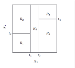
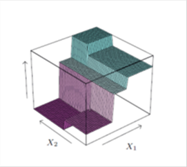
Regression trees are based on the simple idea of recursively partitioning the variable space into increasingly more homogeneous regions. We can visualize the process by limiting the model to two explanatory variables X1 and X2 and a continuous response Y (figure 12, left panel).[27] We first split the space at X1 = t1 and model the response by the mean of Y in each space. Then the region X1 ≤ t1 is split at X2 = t2 and X1 > t1 is split at X1 = t3 and finally X1 > t3 is split at X2 = t4. The result is a partition into 5 regions R1, … , R5 with Y predicted by its constant mean cm in each region (figure 13, right panel). Thus, the continuous explanatory variables are step functions, and the regression model Y = f(X) is based on a simple function I indicating inclusion in the regions.[28]
Figure 12. Partitions by recursive binary splitting based on 2 variables (left) and perspective of response surface (right)
Source: Hastie, Tibshirani, and Friedman, Elements of Statistical Learning, 2009, 321.
A potential problem with regression trees is that the collection of different constant-height regions may inadequately depict the variation in the response surface, especially if the tree (number of regions) is small. Recent boosting algorithms however overcome this problem by estimating many trees (the boost) and averaging them, thereby increasing the granularity of the response surface. Finding the optimal regions is a difficult combinatorial optimization problem that requires the algorithm to find the best variable to split and optimal point in that variable’s range to split; the mean of the response variable in each region is also computed. In the case of a continuous response variable, the algorithm proceeds by minimizing the squared error, or deviance, in a forward stage-wise procedure.[29] At each stage, the algorithm chooses the variable and the split in that variable’s range that most reduces the deviance (Friedman, 2001; Freund and Schapire, 1997; and Friedman, Hastie, and Tibshirani, 2000). The algorithm then proceeds to find the next optimal variable to split and optimal split point and continues until some stopping criterion is met, such as improvement in deviance reduction has ended or a minimum number of observations are at a node.
Overfitting is another potential problem because the algorithm could continue until each response point is in a separate region and a perfect fit is achieved. SBRT modelers view the data as a sample from an unknown underlying distribution and seek to uncover the distribution’s key attributes, so that the model would remain valid when applied to different data.[30] In the statistical learning literature, data are typically divided into a training dataset to estimate key parameters and a test dataset to validate the model. We address the possibility of overfitting by adjusting a shrinkage parameter (explained in the next paragraph) and by removing, or pruning, any variable that does not contribute to the fit. Also, the forward stage-wise procedure will not select a variable unless its inclusion reduces the deviance.
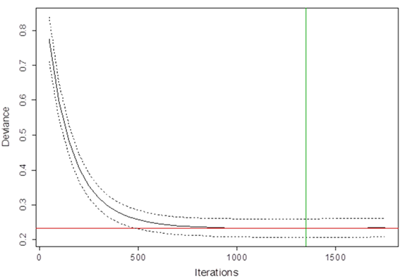
We address the tradeoff between too coarse of a response surface and overfitting by adjusting a shrinkage parameter, which affects the number of iterations and fineness of the response surface, to 0.005.[31] With the shrinkage parameter set, we then estimate the desired number of iterations based on the reduction in deviance by using 5-fold cross validation.[32] The cross-validation deviance initially decreases rapidly, slows, and reaches a minimum of 0.232 with a standard error of 0.026 after 1,350 iterations (figure 14). Repeating iterations beyond the minimum point may introduce noise into the process, and the deviance could eventually increase with more iterations. Thus, the SBRT models in this study are estimated with 1,350 iterations.
Another feature of SBRTs is that a random sample of the full data is drawn at each iteration and used for the calculations during that iteration. Friedman showed that introducing this stochastic component improves the estimates and leads to a more general model (Friedman, 2002). Although small subsamples increase the variance at each iteration, there is less correlation between the estimates at different iterations, which tends to reduce the variance of the combined model. In line with recommendations from the literature, we set the subsampling fraction to 0.5 for SBRT models in this study (Friedman, 2002).
Figure 13 Iterations versus deviance
Source: Authors' calculations.
Appendix B: Prediction
In this appendix, we use the regression model and the SBRT model developed in the report to predict the hours required to produce the 2014 reports. We take the regression model from table 5, column D and re-estimate it using data only through 2013. We take the estimated coefficients from that model and use the values of the explanatory variables for the 2014 projects to predict the hours used to produce those reports. Similarly for the SBRT model, we use the data through 2013 as the training dataset and the explanatory variables for 2014 as the test data to predict hours per report for 2014. The results are fairly close for some reports, but the regression prediction overshoots the hours for India Trade Barriers by a wide margin (table 6). To evaluate the overall performance of the methods, we take simple averages of the observed hours and the predicted hours for the regression and the SBRT models. The simple average of the SBRT predictions is within 67 hours of the observed hours for these reports, but the regression prediction overshoots them by 3,971 hours. In addition, we calculate the mean absolute value of the distance between the predicted and observed values of the individual projects, and the SBRT model performs better than the regression model on this indicator.
Table 6. Observed and predicted total hours of 2014 reports
|
Project title |
Observed |
Predicted (Regression) |
Predicted (SBRT) |
|---|---|---|---|
|
ATPA (2014) |
2,057 |
2,749 |
2,214 |
|
Year in Trade (2013) |
3,929 |
8,648 |
4,692 |
|
Digital Trade II |
16,132 |
22,554 |
15,758 |
|
Effects of EU Trade Barriers on US SMEs |
5,996 |
9,235 |
6,157 |
|
AGOA: Trade and Investment Performance |
8,875 |
12,082 |
9,193 |
|
India Trade Barriers |
23,552 |
36,237 |
22,449 |
|
EU-So. Africa FTA |
1,950 |
3,337 |
2,283 |
|
Recent Trends (2014) |
3,530 |
2,948 |
3,813 |
|
Average |
8,253 |
12,224 |
8,320 |
|
Mean absolute distance* |
4,117 |
437 |
Note: Data about any reports containing classified national security
information have been deleted.
Source: Authors' calculations.* Mean absolute distance = .
References
Ait-Saadi, Ismail and Mansor Jusoh (2011). “What We Know, What We Still Need to Know: the Asian Currency Crisis Revisited.” Asian Pacific Economic Literature 25, iss. 2: 2137.
Bragin, John (2009). Review of Melanie Mitchell’s Complexity: A Guided Tour. https://jasss.soc.surrey.ac.uk/13/2/reviews/3.html
Carter, Tom (2014). An Introduction to Information Theory and Entropy. Mimeo. https://astarte.csustan.edu/~tom/SFI-CSSS/
Damanpour, Fariborz (May 1996). “Organizational Complexity and Innovation: Developing and Testing Multiple Contingency Models.” Management Science 42, no. 5: 693716.
Friedman, Jerome H. (2002). “Stochastic Gradient Boosting.” Computational Statistics and Data Analysis 38, no. 4: 367378.
Friedman, Jerome H (2001). “Greedy Function Approximation: A Gradient Boosting Machine.” The Annals of Statistics 29, no. 5: 11891232.
Halvorsen, Robert and Raymond Palmquist (June 1980). “The Interpretation of Dummy Variables in Semilogarithmic Equations.” The American Economic Review 70, no. 3: 474475.
Hijmans, Robert J., Steven Phillips, John Leathwick, and Jane Elith (2015). “DISMO: Species Distribution Modeling.” R Package Version 1.0-12. https://CRAN-R-project.org/package=dismo.
Johnson, Paul A. and Marcio G.P. Garcia (2000). “A Regression Tree Analysis of Real Interest Rate Regime Changes.” Applied Financial Economics 10: 171176.
Hastie, Trevor, Robert Tibshirani, and Jerome Friedman (2009). The Elements of Statistical Learning: Data Mining, Inference, and Prediction, 2nd Edition. New York: Springer.
Liu, Peng and Zhizhong Li (November 2012). “Task Complexity: A Review and Conceptualization Framework.” International Journal of Industrial Ergonomics 42, iss. 6: 553568.
Maasoumi, Esfandian and Marcelo C. Medeiros (2010). “The Link between Statistical Learning Theory and Econometrics: Applications in Economics, Finance, and Marketing.” Econometric Reviews 29, no. 5: 470475.
Milioris, Dimitrios and Philippe Jacquet (2014). “Joint Sequence Complexity Analysis: Application to Social Networks Information Flow.” Bell Labs Technical Journal 18, no. 4: 7588.
R Core Team (2015). R: A Language and Environment for Statistical Computing. R Foundation for Statistical Computing. Vienna, Austria. https://www.R-project.org/.
Ridgeway, Greg (2015). “GBM: Generalized Boosted Regression Models.” R Package Version 2.1.1. https://CRAN.R-project.org/package=gbm.
Ridgeway, Greg (2012). “Generalized Boosted Models: A Guide to the GBM Package.”
Vrabic, Rok and Peter Butala (2012). “Assessing Operational Complexity of Manufacturing Systems Based on Statistical Complexity.” International Journal of Production Research 50, no 14: 36733685.
Xia, Weidong and Gwanhoo Lee (2005). “Complexity of Information Systems Development Projects: Conceptualization and Measurement Development.” Journal of Management Information Systems 22, no. 1: 4583.
Zeltzer, Luiza, Veronique Limere, Hendrik Van Landeghem, El-Houssaine Aghezzaf, and Johan Stahre (2013). “Measuring Complexity in Mixed-Model Assembly Workstations.” International Journal of Production Research 51, no. 15: 46304643.
Appendix C: Data Used in Figures
Data for Figure 1. Number of reports completed, by year and type, 2014
|
Year |
332 |
103 |
131/2104 |
|---|---|---|---|
|
02 |
18 |
|
2 |
|
03 |
13 |
|
6 |
|
04 |
16 |
4 |
7 |
|
05 |
17 |
3 |
3 |
|
06 |
13 |
2 |
5 |
|
07 |
21 |
4 |
2 |
|
08 |
14 |
3 |
|
|
09 |
12 |
2 |
|
|
10 |
16 |
1 |
1 |
|
11 |
12 |
|
1 |
|
12 |
12 |
1 |
1 |
|
13 |
14 |
1 |
2 |
|
14 |
10 |
|
1 |
Data for Figure 2. Total hours for completed reports, 2002-2014
|
Year |
332 |
103 |
131/2104 |
|---|---|---|---|
|
02 |
78,713 |
|
4,159 |
|
03 |
68,906 |
|
14,784 |
|
04 |
83,083 |
815 |
27,468 |
|
05 |
78,813 |
2,667 |
6,201 |
|
06 |
47,008 |
4,036 |
16,764 |
|
07 |
81,071 |
1,932 |
13,544 |
|
08 |
79,459 |
3,412 |
|
|
09 |
65,364 |
2,879 |
|
|
10 |
77,108 |
805 |
3,560 |
|
11 |
68,538 |
|
1,723 |
|
12 |
69,482 |
601 |
2,002 |
|
13 |
69,975 |
7,785 |
7,354 |
|
14 |
71,726 |
|
2,203 |
Data for Figure 3. Average hours and divisions for completed reports, 2002-2014
|
Year |
Average Hours |
Average Divisions |
|---|---|---|
|
02 |
4,144 |
7.6 |
|
03 |
4,405 |
7.2 |
|
04 |
4,125 |
7.0 |
|
05 |
3,812 |
5.9 |
|
06 |
3,390 |
5.7 |
|
07 |
3,576 |
6.0 |
|
08 |
4,875 |
6.6 |
|
09 |
4,874 |
6.9 |
|
10 |
4,526 |
7.1 |
|
11 |
5,405 |
6.3 |
|
12 |
5,149 |
7.3 |
|
13 |
5,007 |
9.2 |
|
14 |
6,721 |
10.9 |
Data for Figure 4. Trends in report length, 2002-2014
|
Year |
Average |
Average |
Average
|
Average |
|---|---|---|---|---|
|
02 |
168 |
5 |
49 |
198 |
|
03 |
159 |
4 |
55 |
183 |
|
04 |
141 |
5 |
30 |
246 |
|
05 |
152 |
4 |
31 |
181 |
|
06 |
138 |
6 |
35 |
187 |
|
07 |
122 |
4 |
26 |
183 |
|
08 |
160 |
4 |
31 |
215 |
|
09 |
176 |
5 |
54 |
225 |
|
10 |
158 |
5 |
48 |
171 |
|
11 |
168 |
4 |
48 |
199 |
|
12 |
180 |
6 |
46 |
200 |
|
13 |
202 |
5 |
61 |
230 |
|
14 |
211 |
5 |
64 |
240 |
Data for Figure 5. Number of completed reports with standard and advanced CGE analysis, 2002,2014
|
Year |
Standard |
Advanced |
|---|---|---|
|
02 |
6 |
0 |
|
03 |
3 |
0 |
|
04 |
4 |
1 |
|
05 |
0 |
1 |
|
06 |
2 |
1 |
|
07 |
2 |
0 |
|
08 |
0 |
1 |
|
09 |
0 |
2 |
|
10 |
0 |
1 |
|
11 |
0 |
3 |
|
12 |
0 |
1 |
|
13 |
0 |
1 |
|
14 |
0 |
2 |
Data for Figure 6. Number of completed reports with different levels of survey analysis, 2002,2014
|
Year |
Not probability based |
Probability based |
|---|---|---|
|
01 |
1 |
0 |
|
02 |
2 |
0 |
|
03 |
2 |
0 |
|
04 |
1 |
0 |
|
05 |
2 |
0 |
|
06 |
1 |
0 |
|
07 |
3 |
0 |
|
08 |
2 |
0 |
|
09 |
1 |
0 |
|
10 |
0 |
1 |
|
11 |
0 |
1 |
|
12 |
0 |
1 |
|
13 |
0 |
1 |
|
14 |
0 |
2 |
Data for Figure 7. Number of completed reports with different levels of econometric analysis, 2002-2014
|
Year |
Standard |
Moderate |
Advanced |
|---|---|---|---|
|
02 |
0 |
0 |
0 |
|
03 |
0 |
0 |
0 |
|
04 |
0 |
1 |
1 |
|
05 |
2 |
0 |
0 |
|
06 |
0 |
2 |
0 |
|
07 |
0 |
1 |
0 |
|
08 |
0 |
0 |
0 |
|
09 |
0 |
1 |
0 |
|
10 |
2 |
0 |
0 |
|
11 |
0 |
1 |
0 |
|
12 |
0 |
0 |
0 |
|
13 |
2 |
1 |
1 |
|
14 |
0 |
1 |
1 |
Data for Figure 8. Number of completed reports with PE analysis, 2002-2014
|
Year |
PE analysis |
|---|---|
|
02 |
2 |
|
03 |
2 |
|
04 |
4 |
|
05 |
6 |
|
06 |
5 |
|
07 |
6 |
|
08 |
5 |
|
09 |
4 |
|
10 |
2 |
|
11 |
3 |
|
12 |
3 |
|
13 |
3 |
|
14 |
1 |
Data for Figure 9. Relative influence of variables
|
Year |
Relative influence, % |
|---|---|
|
Econometrics |
0.2 |
|
Strategic research. area |
0.3 |
|
Classified |
0.5 |
|
CGE model |
1.1 |
|
PE model |
2.1 |
|
Survey |
2.5 |
|
Type |
2.8 |
|
Appendices |
5.0 |
|
Year |
5.6 |
|
Text pages |
29.4 |
|
Divisions |
50.5 |
Data for Figure 10. Partial influence plots: divisions
|
Divisions |
Total Hours |
|---|---|
|
1.00 |
0.79 |
|
1.16 |
0.79 |
|
1.32 |
0.79 |
|
1.48 |
0.79 |
|
1.65 |
0.90 |
|
1.81 |
0.90 |
|
1.97 |
0.90 |
|
2.13 |
0.90 |
|
2.29 |
0.90 |
|
2.45 |
0.90 |
|
2.62 |
1.28 |
|
2.78 |
1.28 |
|
2.94 |
1.28 |
|
3.10 |
1.28 |
|
3.26 |
1.28 |
|
3.42 |
1.28 |
|
3.59 |
2.21 |
|
3.75 |
2.21 |
|
3.91 |
2.21 |
|
4.07 |
2.20 |
|
4.23 |
2.20 |
|
4.39 |
2.20 |
|
4.56 |
3.06 |
|
4.72 |
3.06 |
|
4.88 |
3.06 |
|
5.04 |
3.07 |
|
5.20 |
3.07 |
|
5.36 |
3.07 |
|
5.53 |
3.20 |
|
5.69 |
3.20 |
|
5.85 |
3.20 |
|
6.01 |
3.20 |
|
6.17 |
3.20 |
|
6.33 |
3.20 |
|
6.49 |
3.20 |
|
6.66 |
3.25 |
|
6.82 |
3.25 |
|
6.98 |
3.25 |
|
7.14 |
3.25 |
|
7.30 |
3.25 |
|
7.46 |
3.25 |
|
7.63 |
3.97 |
|
7.79 |
3.97 |
|
7.95 |
3.97 |
|
8.11 |
3.97 |
|
8.27 |
3.97 |
|
8.43 |
3.97 |
|
8.60 |
3.85 |
|
8.76 |
3.85 |
|
8.92 |
3.85 |
|
9.08 |
3.85 |
|
9.24 |
3.85 |
|
9.40 |
3.85 |
|
9.57 |
4.12 |
|
9.73 |
4.12 |
|
9.89 |
4.12 |
|
10.05 |
4.12 |
|
10.21 |
4.12 |
|
10.37 |
4.12 |
|
10.54 |
5.13 |
|
10.70 |
5.13 |
|
10.86 |
5.13 |
|
11.02 |
5.13 |
|
11.18 |
5.13 |
|
11.34 |
5.13 |
|
11.51 |
5.30 |
|
11.67 |
5.30 |
|
11.83 |
5.30 |
|
11.99 |
5.30 |
|
12.15 |
5.30 |
|
12.31 |
5.30 |
|
12.47 |
5.30 |
|
12.64 |
5.41 |
|
12.80 |
5.41 |
|
12.96 |
5.41 |
|
13.12 |
5.41 |
|
13.28 |
5.41 |
|
13.44 |
5.41 |
|
13.61 |
5.42 |
|
13.77 |
5.42 |
|
13.93 |
5.42 |
|
14.09 |
5.42 |
|
14.25 |
5.42 |
|
14.41 |
5.42 |
|
14.58 |
5.42 |
|
14.74 |
5.42 |
|
14.90 |
5.42 |
|
15.06 |
5.42 |
|
15.22 |
5.42 |
|
15.38 |
5.42 |
|
15.55 |
5.42 |
|
15.71 |
5.42 |
|
15.87 |
5.42 |
|
16.03 |
5.42 |
|
16.19 |
5.42 |
|
16.35 |
5.42 |
|
16.52 |
5.42 |
|
16.68 |
5.42 |
|
16.84 |
5.42 |
|
17.00 |
5.42 |
Data for Figure 10. Partial influence plots: text pages
|
Text pages |
Total Hours |
|---|---|
|
12.00 |
1.30 |
|
17.82 |
1.30 |
|
23.64 |
1.30 |
|
29.45 |
1.30 |
|
35.27 |
1.30 |
|
41.09 |
1.30 |
|
46.91 |
1.60 |
|
52.73 |
1.53 |
|
58.55 |
1.58 |
|
64.36 |
1.62 |
|
70.18 |
2.04 |
|
76.00 |
2.04 |
|
81.82 |
1.98 |
|
87.64 |
2.17 |
|
93.45 |
2.17 |
|
99.27 |
2.22 |
|
105.09 |
2.26 |
|
110.31 |
2.36 |
|
116.73 |
2.45 |
|
122.55 |
2.79 |
|
128.36 |
2.81 |
|
134.18 |
2.92 |
|
140.00 |
2.99 |
|
145.82 |
3.15 |
|
151.64 |
3.28 |
|
157.45 |
3.21 |
|
163.27 |
3.21 |
|
169.09 |
3.14 |
|
174.91 |
3.18 |
|
180.73 |
3.36 |
|
186.55 |
3.85 |
|
192.36 |
3.96 |
|
198.18 |
3.99 |
|
204.00 |
3.88 |
|
209.82 |
3.84 |
|
215.64 |
3.80 |
|
221.45 |
3.79 |
|
227.27 |
3.73 |
|
233.09 |
3.73 |
|
238.91 |
3.73 |
|
244.73 |
3.81 |
|
250.55 |
3.78 |
|
256.36 |
3.71 |
|
262.12 |
3.70 |
|
268.00 |
3.73 |
|
273.82 |
3.79 |
|
279.64 |
3.93 |
|
285.45 |
4.29 |
|
291.27 |
4.37 |
|
297.09 |
4.34 |
|
302.91 |
4.35 |
|
308.73 |
4.34 |
|
314.55 |
4.31 |
|
320.36 |
4.35 |
|
326.18 |
4.39 |
|
332.00 |
4.65 |
|
337.82 |
4.69 |
|
343.64 |
4.69 |
|
349.45 |
4.70 |
|
355.27 |
4.70 |
|
361.09 |
4.70 |
|
366.91 |
4.70 |
|
372.73 |
4.70 |
|
378.55 |
4.70 |
|
384.36 |
4.70 |
|
390.18 |
4.70 |
|
396.00 |
4.70 |
|
401.82 |
4.70 |
|
407.64 |
4.70 |
|
413.45 |
4.70 |
|
419.27 |
4.70 |
|
425.09 |
4.70 |
|
430.91 |
4.70 |
|
436.73 |
4.70 |
|
442.55 |
4.70 |
|
448.36 |
4.70 |
|
454.18 |
4.70 |
|
460.00 |
4.70 |
|
465.82 |
4.70 |
|
471.64 |
4.70 |
|
477.45 |
4.70 |
|
483.27 |
4.70 |
|
489.09 |
4.70 |
|
494.91 |
4.70 |
|
500.73 |
4.70 |
|
506.55 |
4.70 |
|
512.36 |
4.70 |
|
518.18 |
4.70 |
|
524.00 |
4.70 |
|
529.82 |
4.70 |
|
535.64 |
4.70 |
|
541.45 |
4.70 |
|
547.27 |
4.70 |
|
553.09 |
4.70 |
|
558.91 |
4.70 |
|
564.73 |
4.70 |
|
570.55 |
4.70 |
|
576.36 |
4.70 |
|
582.18 |
4.70 |
|
588.00 |
4.70 |
Data for Figure 10. Partial influence plots: year
|
Year |
Total Hours |
|---|---|
|
1.00 |
2.31 |
|
1.13 |
2.31 |
|
1.26 |
2.31 |
|
1.39 |
2.31 |
|
1.53 |
2.31 |
|
1.66 |
2.31 |
|
1.79 |
2.31 |
|
1.92 |
2.31 |
|
2.05 |
2.31 |
|
2.18 |
2.31 |
|
2.31 |
2.31 |
|
2.44 |
2.31 |
|
2.58 |
2.64 |
|
2.71 |
2.64 |
|
2.84 |
2.64 |
|
2.97 |
2.64 |
|
3.10 |
2.64 |
|
3.23 |
2.64 |
|
3.36 |
2.64 |
|
3.49 |
2.64 |
|
3.63 |
2.84 |
|
3.76 |
2.84 |
|
3.89 |
2.84 |
|
4.02 |
2.84 |
|
4.15 |
2.84 |
|
4.28 |
2.84 |
|
4.41 |
2.84 |
|
4.55 |
2.77 |
|
4.68 |
2.77 |
|
4.81 |
2.77 |
|
4.94 |
2.77 |
|
5.07 |
2.77 |
|
5.20 |
2.77 |
|
5.33 |
2.77 |
|
5.46 |
2.77 |
|
5.60 |
3.11 |
|
5.73 |
3.11 |
|
5.86 |
3.11 |
|
5.99 |
3.11 |
|
6.12 |
3.11 |
|
6.25 |
3.11 |
|
6.38 |
3.11 |
|
6.52 |
3.17 |
|
6.65 |
3.17 |
|
6.78 |
3.17 |
|
6.91 |
3.17 |
|
7.04 |
3.17 |
|
7.17 |
3.17 |
|
7.30 |
3.17 |
|
7.43 |
3.17 |
|
7.57 |
3.08 |
|
7.70 |
3.08 |
|
7.83 |
3.08 |
|
7.96 |
3.08 |
|
8.09 |
3.08 |
|
8.22 |
3.08 |
|
8.35 |
3.08 |
|
8.48 |
3.08 |
|
8.62 |
3.20 |
|
8.75 |
3.20 |
|
8.88 |
3.20 |
|
9.01 |
3.20 |
|
9.14 |
3.20 |
|
9.27 |
3.20 |
|
9.40 |
3.20 |
|
9.54 |
3.14 |
|
9.67 |
3.14 |
|
9.80 |
3.14 |
|
9.93 |
3.14 |
|
10.06 |
3.14 |
|
10.19 |
3.14 |
|
10.32 |
3.14 |
|
10.45 |
3.14 |
|
10.59 |
3.27 |
|
10.72 |
3.27 |
|
10.85 |
3.27 |
|
10.98 |
3.27 |
|
11.11 |
3.27 |
|
11.24 |
3.27 |
|
11.37 |
3.27 |
|
11.51 |
3.10 |
|
11.64 |
3.10 |
|
11.77 |
3.10 |
|
11.90 |
3.10 |
|
12.03 |
3.10 |
|
12.16 |
3.10 |
|
12.29 |
3.10 |
|
12.42 |
3.10 |
|
12.56 |
2.97 |
|
12.69 |
2.97 |
|
12.82 |
2.97 |
|
12.95 |
2.97 |
|
13.08 |
2.97 |
|
13.21 |
2.97 |
|
13.34 |
2.97 |
|
13.47 |
2.97 |
|
13.61 |
2.97 |
|
13.74 |
2.97 |
|
13.87 |
2.97 |
|
14.00 |
2.97 |
Data for Figure 10. Partial influence plots: appendices
|
Appendices |
Total Hours |
|---|---|
|
0.00 |
2.41 |
|
0.15 |
2.41 |
|
0.30 |
2.41 |
|
0.45 |
2.41 |
|
0.61 |
2.40 |
|
0.76 |
2.40 |
|
0.91 |
2.40 |
|
1.06 |
2.40 |
|
1.21 |
2.40 |
|
1.36 |
2.40 |
|
1.52 |
2.60 |
|
1.67 |
2.60 |
|
1.82 |
2.60 |
|
1.97 |
2.60
|
|
2.12 |
2.61 |
|
2.27 |
2.61 |
|
2.42 |
2.61 |
|
2.58 |
2.94 |
|
2.73 |
2.94 |
|
2.88 |
2.94 |
|
3.03 |
2.95 |
|
3.18 |
2.95 |
|
3.33 |
2.95 |
|
3.48 |
2.95 |
|
3.64 |
3.02 |
|
3.79 |
3.02 |
|
3.94 |
3.02 |
|
4.09 |
3.02 |
|
4.24 |
3.02 |
|
4.39 |
3.02 |
|
4.55 |
3.12 |
|
4.70 |
3.12 |
|
4.85 |
3.12 |
|
5.00 |
3.12 |
|
5.15 |
3.12 |
|
5.30 |
3.12 |
|
5.45 |
3.12 |
|
5.61 |
3.11 |
|
5.76 |
3.11 |
|
5.91 |
3.11 |
|
6.06 |
3.11 |
|
6.21 |
3.11 |
|
6.36 |
3.11 |
|
6.52 |
3.19 |
|
6.67 |
3.19 |
|
6.82 |
3.19 |
|
6.97 |
3.19 |
|
7.12 |
3.19 |
|
7.27 |
3.19 |
|
7.42 |
3.19 |
|
7.58 |
3.22 |
|
7.73 |
3.22 |
|
7.88 |
3.22 |
|
8.03 |
3.22 |
|
8.18 |
3.22 |
|
8.33 |
3.22 |
|
8.48 |
3.22 |
|
8.64 |
3.22 |
|
8.79 |
3.22 |
|
8.94 |
3.22 |
|
9.09 |
3.22 |
|
9.24 |
3.22 |
|
9.39 |
3.22 |
|
9.55 |
3.22 |
|
9.70 |
3.22 |
|
9.85 |
3.22 |
|
10.00 |
3.22 |
|
10.15 |
3.22 |
|
10.30 |
3.22 |
|
10.45 |
3.22 |
|
10.61 |
3.22 |
|
10.76 |
3.22 |
|
10.91 |
3.22 |
|
11.06 |
3.22 |
|
11.21 |
3.22 |
|
11.36 |
3.22 |
|
11.52 |
3.22 |
|
11.67 |
3.22 |
|
11.82 |
3.22 |
|
11.97 |
3.22 |
|
12.12 |
3.22 |
|
12.27 |
3.22 |
|
12.42 |
3.22 |
|
12.58 |
3.22 |
|
12.73 |
3.22 |
|
12.88 |
3.22 |
|
13.03 |
3.22 |
|
13.18 |
3.22 |
|
13.33 |
3.22 |
|
13.48 |
3.22 |
|
13.64 |
3.22 |
|
13.79 |
3.22 |
|
13.94 |
3.22 |
|
14.09 |
3.22 |
|
14.24 |
3.22 |
|
14.39 |
3.22 |
|
14.55 |
3.22 |
|
14.70 |
3.22 |
|
14.85 |
3.22 |
|
15.00 |
3.22 |
Data for Figure 11. Partial influence: categorical
|
Variables |
Effect on hours |
|---|---|
|
Project type = 103 |
-0.02 |
|
Project type = 131/2104 |
-0.13 |
|
Project type = 332 |
0.15 |
|
Survey = no |
-0.16 |
|
Survey = year |
0.16 |
|
PE model = no |
0.17 |
|
PE model = yes |
-0.08 |
|
CGE model = none |
0.01 |
|
CGE model = standard |
-0.09 |
|
CGE model = advanced |
0.07 |
|
Classified = no |
-0.03 |
|
Classified = year |
0.03 |
|
Strategic research area = no |
-0.03 |
|
Strategic research area = yes |
0.03 |
|
Econometrics = no |
-0.02 |
|
Econometrics = yes |
0.02 |
Note:
the y-axis is the log of total hours per report, and the estimates are scaled
so that the estimated effects of the different levels of each variable sum to
zero. Variables with large differences between their levels are relatively more
influential. Letting D equal the difference in levels, the percentage effect on
hours of the different levels of a variable equals
Data for Figure 12. Partitions by recursive binary splitting based on 2 variables (left) and perspective of response surface (right)
This figure is a stylized diagram without numbers. See alternative text for description.
Data for Figure 13. Iterations versus deviance
This figure reports the results of a convergence procedure. The figure has 1,750 points and the data representation require 10 pages (eight columns per page). The alternative text provides an accurate succinct description.
[1] USITC, Annual Performance Report, FY 2014.
[2] A division is one of the lowest level organizational units at the Commission. Each division has a chief who reports to an office director. A division’s responsibilities can be either topical, as the Services Division in the Office of Industries, or functional, as the Research Division in the Office of Economics. Around 10 people typically comprise a division although actual numbers vary.
[3] Commissioners and their staff began charging hours to projects during the time that these data were collected. To assure data consistency, this study excludes their time.
[4] Data on labor costs became available in late 2001 and therefore dictate the starting year. The first full year of data is 2002.
[5] The original data list some investigations twice because they were instituted under dual authorities and other recurring investigations, such as Year in Trade, are only listed once, even though there are multiple reports. For this research, we focus on the reports and have a unique entry for each report produced between 2002 and 2014.
[6] We use “type of report” to refer to the different authorities under which an investigation is carried out. For example, a 332 report, which is instituted under section 332 of the Tariff Act of 1930, is a general investigation on any matter involving tariffs or trade. These tend to be the Commission’s most variable and complex reports. Investigations of the probable economic effects of trade agreements are instituted under section 131 of the Trade Act of 1974 and section 2104 of the Trade Act of 2002. Section 103 reports are more narrowly defined studies of the probable economic effects of tariff modifications. There is variation within these overall types of reports that affect their complexity. Other reports are produced under different authorities. For this research, we group the Year in Trade reports with the 332 reports.
[7] Because recurring reports always have the same labor code, we give them special attention and link them to specific reports according to when the hours are charged to the relevant labor code. Non-recurring reports do not have this problem because their labor codes are only used for one report.
[8] This is the length of the pdf file, which includes non-content pages such as front materials and blank pages. We assume that these types of pages are approximately the same in all reports.
[9] The number of countries is determined by counting the number of countries listed in the table of contents. Regions, such as the EU, are counted as one rather than 28 in this example.
[10] Areas of strategic research change over time and have included foreign direct investment, computable general equilibrium modeling, environment and renewable energy, emerging markets, and nontariff measures. A new approach is a previously unused method or way of obtaining or analyzing information for a report. An example is the use of roundtables to gather information for a project related to small businesses exporting to the EU. Another example is the analysis of Indian industrial policies using the theory of economic complexity. Obtaining information on these variables relied on the subjective judgment of the authors or subject-area experts.
[11] The standard level would be a straightforward application of an existing CGE model, such as in the report U.S.-Colombia Trade Promotion Agreement: Potential Economy-wide and Selected Sectorial Effects (2104-023). The advanced level could involve creating a new baseline for an existing model or calibrating a new model.
[12] A standard level would use summary statistics, correlation coefficients, or regression model that one might find in an introductory trade textbook. A moderate level could be an advanced gravity model or regression specification similar to the analysis in the Environmental Services study in 2012, which used a Poisson regression. A difficult level, while relatively rare, would be similar to the regression analysis used in the Olive Oil 332 study, which estimates demand for olive oil from retail scanner data based on a demand-systems approach.
[13] This reduction in data occurs for a variety of reasons, with incorrect or missing labor cost data being the primary reason. Some investigations were canceled or the labor cost system was implemented after the report had begun. Three reports were dropped for the following other reasons: 1. Shifts in U.S. Merchandise Trade 2011 only consists of tables and is not representative of the other reports in this recurring series. 2. U.S. Trade and Investment with Sub-Saharan Africa: Fifth Annual Report appears to have been active from May 2000 to December 2004 and spans a period before the labor cost system was implemented. 3. The Textiles and Apparel Monthly report does not conform with other reports in the database and monthly hours would be inaccurate because pay periods do not align with the beginning and end of a month.
[14] These studies take on average 106 days whereas 332 studies on average take 265 days. In the interest of parsimony, all 2104 reports whether produced separately or in a joint 131-2104 investigation are included in the 131/2104 grouping.
[15] The percentage effect of an indicator variable on the response variable equals 100(eβ-1). See Halvorsen and Palmquist (1980).
[16] As explained in the background section, we assume that the requestor or the topic addressed exogenously determines the scope of the report and that the personnel who happen to be available at the time do not dictate the level of analysis or the use of advanced techniques.
[17] Honda Lagrange multiplier tests indicate the presence of substantial heterogeneity from year to year, and we therefore add yearly fixed effects.
[18] Breusch-Pagan tests reveal the presence of heteroskedasticity, although plots of the residuals do not show that it is severe. Breusch-Godfrey tests for serial correlation show that it is present in most runs.
[19] Ramsey reset tests are calculated and show that the models are consistent with the hypothesis of no misspecification. Q-Q plots of the residuals show them to be approximately normally distributed.
[20] Thus, one could take logarithms of both sides and attempt to estimate the resulting equation, but it would be meaningless because the equation is perfectly collinear, and the coefficient estimates would be one, the R2 would be one, and the standard errors would be undefined. Estimation will still succeed if collinearity is high but not perfect, although the standard errors will be large. We monitor collinearity by computing the condition number of the regression matrix and avoiding combinations of explanatory variables that are highly collinear.
[21] The report type variable appears to capture generic differences in complexity among these different types of reports; the adjustment mentioned in footnote 15 is used for the calculation.
[22] For example, see Ait-Saadi and Jusoh, “What We Know, What We Still Need to Know, 2011;” Maasoumi and Medeiros, “The Link between Statistical Learning Theory and Econometrics,” 2010; and Johnson and Garcia, “A Regression Tree Analysis of Real Interest Rates,” 2000.
[23] The SBRT model is implemented in R (R Core Team, 2015) using the GBM package (Ridgeway, 2015) and the DISMO package (Hijmans et al., 2015).
[24] This includes leaving the response variable hours per report in logs.
[25] The estimate for PE model was not significant in the regression analysis; results concerning CGE analysis are similar in both the regression and the SBRT models.
[26] In addition, with the exception of 2013, relatively few studies have incorporated econometric analysis, which doubtlessly contributes to its small influence on hours per report.
[27] The example is from Hastie, Tibshirani, and Friedman, Elements of Statistical Learning, 2009, 321.
[28] A tree diagram with a branch at each partition could also represent the modelhence the name regression tree. Such a diagram quickly becomes congested if there are many partitions, and these diagrams are seldom used with SBRT models in practice.
[29] This is somewhat analogous to forward stepwise regression. The definition of deviance in the context of SBRTs varies, depending on the loss function and its gradient. In this case with a continuous response variable, we use a squared loss function with Gaussian errors, and the deviance is a squared error term.
[30] In this sense, regression and SBRTs may have different goals, as regression analysis generally aims to discover the strongest relationship among a single set of data. The possibility of continuing the algorithm until a perfect fit is achieved makes goodness-of-fit statistics, such as an R2 less important to SBRT modeling, which is more concerned about how the model performs when confronted with new data.
[31] Based on Monte Carlo simulations, researchers recommend a shrinkage rate of between 0.01 and 0.001, with smaller values providing better predictive performance. Ridgeway, “Generalized Boosted Models: A Guide to the GBM Package,” 2012.
[32] In 5-fold cross validation, the sample is randomly partitioned in 5 subsamples of equal size, and four subsamples are used as the training data and the other is the test data. Estimation is repeated 5 times, so that each subsample is used once as the test data. The results are then averaged. Ridgeway tested various methods for selecting the optimal number of iterations across 13 real datasets and found 5-fold cross validation to be the best approach. Ridgeway, “Generalized Boosted Models: A Guide to the GBM Package,” 2012, 9.