Figure 1: PQV index (weighted median and IQR) by HS summary sections

One-Way and Two-Way Chinese Trade
William Deese
ECONOMICS WORKING PAPER SERIES
Working Paper 2017–05–D
U.S. INTERNATIONAL TRADE COMMISSION
500 E Street SW
Washington, DC 20436
May 2017
Office of Economics working papers are the result of ongoing professional research of USITC Staff and are solely meant to represent the opinions and professional research of individual authors. These papers are not meant to represent in any way the views of the U.S. International Trade Commission or any of its individual Commissioners. Working papers are circulated to promote the active exchange of ideas between USITC Staff and recognized experts outside the USITC and to promote professional development of Office Staff by encouraging outside professional critique of staff research.
One-Way and Two-Way Chinese Trade
William Deese
Office of Economics Working Paper 2017–05–D
May, 2017
Abstract
This study decomposes China’s total trade into one-way trade (also called interindustry trade) and two-way trade (also called intra-industry trade). One-way trade accounts for the major share of China’s trade. The share of two-way trade where China’s exports are priced less than its imports of similar products grew over the past two decades. Indexes are created that show differences in capital-labor ratios, economic size, similar stage of development, workforce skill level, and trade costs between China and its trade partners. These indexes are used in a logit model to explain the probability of the occurrence of two-way trade and in another regression to explain the relative unit values of Chinese exports and imports when there is two-way trade. A large panel dataset based primarily on Chinese customs data is used, and the estimation incorporates large numbers of fixed effects. Many of the explanatory variables are statistically significant including types of Chinese trading firms, the labor-skill index, the capital-labor ratio, stage of development, and economic size.
William Deese
Research Division
Office of Economics
U.S. International Trade Commission
william.deese@usitc.gov
Grubel and LLoyd [13] were pioneers in systematically quantifying intraindustry trade—simultaneously exporting and importing similar goods. While their type of decomposition of a country’s entire goods trade has some intrinsic merit, its greatest value lies in possible connections with other economic variables of interest. For example, it has been suggested that most trade between similar countries is intra-industry trade, which may not lead to income redistribution. In addition, intraindustry trade may not require reallocations of labor and capital and could therefore be less disruptive than increasing trade in different products where capital and labor are reallocated among industries. Although Grubel and Lloyd formalized these ideas in the 1970s, work based on their ideas continues to the present. I apply concepts similar to Grubel and Lloyd’s approach to analyze Chinese trade. China is an interesting subject of study because its exports grew more than five-fold between 2001, when it acceded to the World Trade Organization, and 2015, and it is currently the world’s largest single country exporter.1 China’s imports also grew substantially, increasing more than four-fold during this period.
This paper seeks to understand Chinese trade patterns by decomposing them into interindustry trade or one-way trade (OWT), where only exports or only imports occur in the same product category, and into intra-industry trade or two-way trade (TWT), where exports and imports simultaneously occur in the same product category. To make concepts totally clear, consider the following example. If men’s dress shirts are a product category and China’s exports of these shirts are offset by similar imports, China has TWT in men’s dress shirts. If China just exports these shirts or just imports them, with no offsetting trade in the same category, there is OWT in this category. After classifying these types of trade, TWT is then further classified into horizontal and vertical components based on differences in unit values between exports and imports. In addition, variables that may determine these types of trade, such as differences in capital-labor ratios, trade costs, etc. are examined via a large panel dataset.
Results show that most Chinese trade is OWT and that the shares of OWT have been steady over the past two decades. The variety of products traded increased for both OWT and TWT, but the increase was relatively greater for TWT. The share of China’s TWT in which its exports are priced lower than its imports grew over the past two decades, and the shares of other types of TWT declined. Chinese processing trade has a greater probability of being OWT, but a trade by a foreign invested firm has a greater probability of being TWT. More similar per capita income between China and its trade partners increases the probability of a trade being two-way. Greater differences in capital-labor ratios between China and its trade partners appear to increase the probability of TWT by a small amount but not to have much effect on the relative price of China’s exports and imports of similar products.
This paper is organized into main sections on background, data, classifying Chinese exports and imports, and econometrics. The background section describes the context in which studies of OWT and TWT occur, including explaining the existence of OWT and TWT, measurement issues, and empirical studies. Then, after the data used in this study are described, the section on classifying Chinese trade breaks Chinese trade into OWT and TWT and further breaks out the components of TWT. Next, the econometric section examines factors that may determine the different types of trade. In addition, the final section concludes.
Grubel and Lloyd [13] were pioneers in the measurement of trade patterns in the 1970s when the Heckscher-Ohlin model founded on differences in factor endowments was the dominant trade theory. Originally a two-country, two-good model, it states that trade occurs when one country exports the good that uses its abundant factor intensively in production and imports the good that uses its scarce factor intensively. Thus, a capital abundant country would export capital-intensive goods and import labor-intensive goods. In this way, trade leads to a more efficient allocation of resources, in which the abundant factor gains through reallocation, but the factor used in the industry contested by imports is harmed. Thus, goods trade because it leads to factor reallocations could be viewed as trade in the services of factors of production. Although differences in factor endowments no longer have such a dominant position in trade theory, they are still believed to explain much of the trade between countries with large differences in factor endowments. Helpman and Krugman [15] state that despite the existence of TWT, OWT is positively related to the difference in factor endowments between trade partners.
Intra-industry or TWT can be explained in a variety of ways. One view is that industries use similar production technologies to produce a variety of goods. A version of this approach is that every firm chooses a unique variety and prices it to maximize profits. If consumers either like variety or different people like different goods and there are increasing returns to scale, firms have incentives to expand internationally. In this setup, one would expect to find goods produced with similar factor proportions being exchanged internationally. Countries with identical relative factor endowments would only engage in intra-industry trade where different varieties of similar products are traded. Consumers including producers using imported intermediate goods benefit from gains in variety. Thus, in this view, TWT increases as relative factor endowments become more similar.2
Davis [6] develops another explanation of intra-industry trade by extending the standard Heckscher-Ohlin model to include Ricardian elements in which differences in technology matter between countries. In this constant returns to scale setting, TWT arises in response to small technical differences among the many products, and specialization develops based on these differences. In addition, Fontagné and Freudenberg [10] show that two-way flows of homogeneous products can occur without product differentiation if markets are highly concentrated.
Early studies of intra-industry trade mainly contrasted it to interindustry trade and did not classify it into horizontal and vertical types. Falvey [8] developed a model in which higher quality products are produced using more capital per unit of labor and consumers prefer different qualities and some are able to pay for higher quality products. In this view, differences in technology or endowments between countries lead to the exchange of higher and lower quality varieties of similar products at different prices (vertically differentiated intra-industry trade).3
One of the most widely used measures of intra-industry trade is the Grubel-LLoyd index. Intra-industry trade at industry or product level i equals total trade (exports plus imports) minus net exports . Grubel and Lloyd [13] note that these measures can be calculated at the industry level or at a higher level of aggregation such as a country level with all or some subset of its trade partners. The following is often referred to as the Grubel-Lloyd index and measures average intra-industry trade as a share of total trade.
| (1) |
When exports exactly match imports, this value equals 1; when there are exports but no imports, or vice versa, this measure is 0. For this expression to measure the share of intra-industry trade accurately, exports and imports must be valued on the same basis; otherwise, the possibility of exports equaling imports is skewed. Because trade statistics typically value exports on a f.o.b. basis and imports on a c.i.f. basis, an adjustment must be made, which many investigators have failed to do. On a related issue, the Grubel-LLoyd index is also distorted if trade is unbalanced because then exports and imports cannot possibly be equal, and total intra-industry trade becomes unattainable. Grubel and Lloyd proposed an alternative measure to employ when exports and imports are out of balance, but Fontagné and Freudenberg [10] as well as others have noted that the alternative approach does not measure intra-industry trade as a share of total trade. They then note that most researchers therefore continue to use the original index.
Fontagné and Freudenberg [10] observe other potential problems with the Grubel-LLoyd index. If countries are assembled into regions before the index is calculated, one country’s interindustry flows of goods could show up as intra-industry flows on a regional basis. Fontagné and Freudenberg show that one can avoid this geographic bias by carrying out research on a strictly bilateral basis. Along similar lines, they note that highly aggregated product or industry data will result in more intra-industry trade than would be the case if more product-specific data were used. Within an industry, the simultaneous export and import of products at different stages of production should not be considered as intra-industry trade. For example, the exchange of motors is not equivalent to the exchange of complete cars. In terms of individual products, the most objective picture emerges if data at the most disaggregated product level are used. Making these simple adjustments, which recent researchers tend to do, shows that intra-industry trade is often less than half of all trade, although Fontagné and Freudenberg find it to be slightly more than half among similar countries in the EU. In contrast, the early work of Grubel and Lloyd, which used more aggregated data (3-digit SITC codes), found that intra-industry trade represented 63 percent of the value of total trade in OECD countries.
In response to these issues, Abd-el-Rahman [19], Fontagné and Freudenberg [10], Fukao et al. [11], Azhar and Elliott [2], and others have developed approaches for decomposing trade, which I adopt, that resolve some of these issues.4 As explained in the next section, I use the most detailed product-level data available on a bilateral basis. The first step is separating OWT from TWT. As will become apparent, it is impossible to eliminate all arbitrariness regardless of the approach. For example, OWT can be defined by examining the value of the minimum flow (export or import) of a product i, with country j, at time t, relative to the corresponding maximum flow (export or import). Here, one faces a choice whether to adopt a strict definition of OWT and include only categories where there is absolutely no trade in the corresponding export or import category, or take a more flexible approach where alpha is greater than 0 in the following equation.
| (2) |
Because trade occurs for many reasons, some researchers, such as Fontagné and Freudenberg, use alphas greater than zero in order to eliminate small incidental trade where the minority flow is only a small share of the majority flow. However, as Azhar and Elliott point out, care should be exercised in order not to exclude important volumes of trade.
There is an extensive literature on intra-industry trade, and several researchers have investigated this topic in an Asian context. Xing [23] finds that most trade between China and Japan and between China and the United States is the interindustry type. Intra-industry trade between China and Japan was only about 6 percent of total trade in 1980 but rose to about a third of trade between these two countries in 2004. In contrast, bilateral trade between China and the United States only increased a few percentage points and remained around 10 percent in 2004. Intra-industry trade between China and the United States was greatest in the chemical sector and lowest in metals and machinery. Intra-industry trade between China and Japan was very low for the food sector but moderate in the metals, chemicals, electrical, and machinery sectors.
Sawyer et al. [20] investigate intra-industry trade in 22 Asian countries using 2003 data and find levels of intra-industry trade at the country-wide level to range between 1.0 percent and 54.0 percent, with higher income countries in East Asia having more intra-industry trade. Zhang et al. [24] use trade data between China and selected European countries and between China and the United States to classify pharmaceutical products into interindustry and intra-industry trade. They find approximately half of this trade to be the intra-industry type. Zheng and Qi [25] investigate the structure of Chinese-U.S. agricultural trade between 1996 and 2005 and find that it is mostly interindustry trade. Fukao et al. [11] investigate trade patterns in East Asia and find that total intra-industry trade in the region grew from 16.6 percent in 1996 to 23.7 percent in 2000, with intra-industry trade where unit values are different (vertical intra-industry trade) growing by slightly more.
Once OWT is defined where there is no significant trade overlap and removed, TWT in similar products remains. Researchers have used differences in unit values between exports and imports to decompose TWT into horizontal trade with small unit-value differences and vertically differentiated products with large differences in unit values. Azhar and Elliott [2] have perhaps the most developed method for this decomposition. Their approach is based on mapping differences in unit values for exports () and imports () into the PQV index that varies between 0 and 2, as shown next.
| (3) |
The PQV index is one when the unit values of exports and imports are equal; is less than one when the unit value of exports is less than that the unit value of imports, and greater than one when the unit value of exports exceeds than that of imports.5 In an upcoming section, I calculate the PQV index for TWT and define low vertical intra-industry trade (VIT-L), horizontal intra-industry trade (HIT), and high vertical intra-industry trade as follows based on the values of the PQV index and where is a range indicating small differences in price, which implies similar products at roughly similar qualities.
| (4) |
The following equation summarizes the relationship between total trade (TT) and OWT, as defined by equation 2, and TWT and its components, as defined by equation 4.
| (5) |
Various researchers have investigated factors influencing TWT. For example, Bergstrand and Egger [4] develop a theoretical and empirical model of TWT that includes trade costs based on cif-fob margins. They find a significant negative relationship between trade cost and the share of TWT, using a cross section of averaged data for OECD countries between 1990 and 2000. They find the expected negative relationship between differences in factor endowments or capital-labor ratios and TWT. They find a significant positive relationship between economic size, based on GDP and the share of TWT. Their measure for similarity of GDPs is not statistically significant.
Martín-Montaner and Orts [17] examine the determinants of vertical TWT between Spain and 20 OECD countries from 1988 to 1992. In contrast to Bergstrand and Egger, they a find positive relationship between the difference in capital-labor endowments and vertical TWT. After constructing indexes for technology stock using OECD science and technology statistics and human capital using years of schooling, they also find positive relationships between these variables and the share of TWT.
Fukao et al. [11] look at the determinants of TWT in Japan’s electrical machinery industry using Japanese Customs data at the HS9 level for 1988. Using a model that includes regional fixed effects, they find that foreign direct investment has a strong positive effect on Japanese TWT in this industry. They find that vertical TWT is lower, the greater the difference in factor endowments, but they find that the difference in factor endowments increases when the gap in per capita GDP between Japan and its trade partners exceeds 10,000 international dollars. They also find that most growth in TWT has been in vertical TWT instead of in horizontal TWT. They use distance as the measure of trade costs and find it to have a statistically significant negative impact. Their results for differences in human capital is not significant.
The contribution of this paper is that it comprehensively investigates patterns in all categories of merchandise and agricultural trade at a highly disaggregated level between China and its trade partners between 1995 and 2015, a 21-year period during which China acceded to the WTO. It also decomposes intra-industry trade into classes based on unit-values that may reflect differences in quality. The econometric analysis assembles a large panel dataset and examines the determinants of China’s TWT and the determinants of the relative unit values of Chinese exports and imports.
Chinese Customs Data, which account for all goods that pass into or out of China’s custom territory, are the main data source. These proprietary data have been used by various researchers. I use annual value and quantity of exports and imports and source and destination countries from 1995 to 2015. These are not firm-level data but some information is included about the trading firms. I use customs regimes and firm or ownership types. The data contain a variety of other information, such as customs district, which I sum out and do not use.
Similar to most countries, China uses the Harmonized Commodity Description and Coding System (HS), an international system to classify traded goods. The World Customs Organization maintains the system, which places similar products close to each other in the numbering scheme. The system is hierarchical in the sense that more detailed product descriptions are contained within the same broad category. For example, a specific two-digit HS code (HS2) contains all products at a HS4 level that share those same first two digits. The Chinese Customs Data are at the HS8 level, which add a couple of thousand more product groups beyond the HS6 data that are available for most countries through UN Comtrade.6
Because it is impractical to report data at the HS8 level of detail, I provide several summaries. One summary is based on HS sections, which present all HS products in 21 sections.7 Another summary is based on broad economic categories (BEC) set forth by the UN Statistical Division. The BEC distinguish economically important groups of commodities, such as food, industrial inputs, capital equipment, consumer durables, and consumer non-durables.8 I also summarize the data geographically by regions.
Chinese customs data have their own country codes whereas most international datasets use ISO codes. I concord these country codes in order to merge other international data with the Chinese data.9 I extract data on total labor force, gross fixed capital formation, GDP, and per capita GDP at purchasing power parity from the World Bank’s World Development Indicators. From the UN Human Development Index, I extract data on average years of school. These data are generally available for the countries and time period in the Chinese Customs Data, although missing values are fairly common and shrink the effective size of the merged dataset when observations with missing data are removed.
Despite some criticism of the use of cif-fob margins as indicators of trade costs, Bergstrand and Egger [4] defend their use, stating that research shows them to be correlated with true trade costs and that practical alternatives are lacking. Although long recognized as potentially useful, inconsistencies have made these margins less useful. For example, for the same good and transport route, the source country fob export value sporadically exceeds the cif import value at the destination port, which includes that export value plus charges for insurance and freight.10 Now, however, OECD researchers have cleaned these data and removed inconsistencies. For product-country combinations with inconsistencies, they estimated replacement values with a gravity equation. The result is the OECD’s Database on International Transport and Insurance Costs, which is at the HS-4 level for a large number of countries from 1995–2014.11 These data are not ideal for my purposes because the product data are at the HS8 level. Nevertheless, due to their consistency, I use them as indicators of trade costs and to put the Chinese values for exports and imports on an equal footing for trade pattern analysis. In addition, I project the cif-fob margins to 2015 using a first order autoregressive process for each product-country combination in order to use them with the other data that extend to 2015.
This section uses Chinese Customs data and applies previously developed concepts to break out Chinese OWT and TWT. All calculations are originally made at the HS-8 level of product detail on a bilateral basis, unless otherwise noted. Once these calculations are made, the data are summarized in different ways to provide a picture of key aspects of the patterns of Chinese trade. First, OWT is described along several dimensions. Next, TWT is identified and further classified as VIT-L when unit values of Chinese exports are significantly below those of corresponding imports, HIT when unit values of exports and imports are about the same, or VIT-H when unit values of Chinese exports are substantially above those of corresponding imports.
As stated in the introduction, Chinese trade grew substantially during the past couple of decades. Total Chinese trade (exports plus imports) experienced double digit growth rates during much of the 2000s; the median annual growth rate was 18.1 percent for these 21 years from 1995–2015 (table 1).12 Despite the strong growth in most years, a small decline occurred in 1998, and larger declines took place in 2009 and 2015. As expected, exports outpaced imports each year and were consistently around 55 percent of total trade.
| Year | TT growth rate | TT export share | GL index | GL index |
| 1995 | – | 53.7 | 25.9 | 11.8 |
| 1996 | 3.3 | 52.8 | 25.4 | 12.1 |
| 1997 | 10.8 | 57.4 | 26.0 | 12.0 |
| 1998 | -0.5 | 57.9 | 26.0 | 12.4 |
| 1999 | 11.5 | 55.2 | 27.0 | 13.0 |
| 2000 | 30.7 | 53.9 | 28.1 | 12.9 |
| 2001 | 7.2 | 53.7 | 27.5 | 13.0 |
| 2002 | 20.9 | 54.1 | 28.7 | 13.3 |
| 2003 | 35.8 | 53.5 | 29.0 | 12.6 |
| 2004 | 35.0 | 53.4 | 29.4 | 12.7 |
| 2005 | 23.4 | 55.6 | 29.5 | 12.4 |
| 2006 | 23.8 | 57.2 | 30.6 | 12.2 |
| 2007 | 23.3 | 58.1 | 29.6 | 11.9 |
| 2008 | 18.1 | 57.7 | 28.5 | 11.3 |
| 2009 | -13.9 | 56.3 | 28.8 | 10.9 |
| 2010 | 33.2 | 55.2 | 27.8 | 10.7 |
| 2011 | 22.0 | 54.3 | 26.8 | 10.2 |
| 2012 | 4.0 | 55.2 | 26.3 | 10.0 |
| 2013 | 5.9 | 55.1 | 26.1 | 9.8 |
| 2014 | 5.5 | 56.5 | 25.8 | 10.1 |
| 2015 | -8.5 | 59.8 | 27.2 | 10.8 |
| Median | 18.1 | 55.2 | 27.4 | 12.0 |
| IQR | 19.0 | 3.3 | 2.8 | 1.9 |
OWT is the most significant component of Chinese trade, and it has fluctuated little over the past couple of decades. Depending upon whether the aggregation is at the HS8 level (next to last column) or at both the HS8 and country level (last column), Grubel-Lloyd indexes show that only slightly more than 10 percent or slightly more than a quarter of Chinese trade is intra-industry trade (TWT). As stated earlier, when the product categories are highly disaggregated and bilateral trade partners are distinguished, the trade overlap or level of intra-industry trade is fairly small. Another important feature of these data is that the trade share and Grubel-Lloyd indexes are much more stable than the annual growth rate of total Chinese trade. Despite the volatility in trade values, the Grubel-Lloyd indices remained in a fairly narrow range, as indicated by their fairly small inter-quartile ranges (IQR).13
As previously explained, strict OWT implies absolutely no corresponding imports or exports, or it can be defined more flexibly. Table 2 shows calculations of OWT on a strict basis and where the minimum flow is less than or equal to 100 times the maximum flow; thus, with = 0.01 in equation 2. Other researchers have often used larger break points; for example, Fontagné and Freudenberg used an alpha of 0.10 in studying inter-European trade. Using a small alpha, such as 0.01, helps assure that only incidental TWT is included with OWT. Still, even though the minority flow is very small relative to the majority flow, there are many instances of these very small flows. Collectively, the change from the strict definition significantly affects the total value of OWT, moving the overall shares of OWT from around a half to around three quarters of total trade. Experimentation shows that increasing alpha to 0.05 (not shown) does not greatly increase the share of OWT beyond the level where alpha equals 0.01. The IQR for these shares is relatively small, ranging from about 3 percent to around 5 percent, indicating little variability. Thus, for subsequent calculations, I settle on the definition of OWT with alpha equal 0.01.
| Strict | Strict | OWT | OWT | Unique HS8 | Unique HS8 | |
| OWT | OWT | 0.01 | 0.01 | categories | categories | |
| Year | exports | imports | exports | imports | exports | imports |
| % | % | % | % | count | count | |
| 1995 | 45.7 | 59.0 | 76.3 | 76.3 | 6028 | 6171 |
| 1996 | 47.9 | 57.8 | 76.1 | 75.4 | 6174 | 6340 |
| 1997 | 49.9 | 56.7 | 77.2 | 72.5 | 6291 | 6362 |
| 1998 | 50.5 | 54.5 | 76.8 | 72.5 | 6479 | 6624 |
| 1999 | 49.1 | 52.2 | 75.8 | 71.9 | 6515 | 6586 |
| 2000 | 49.9 | 54.3 | 75.8 | 73.8 | 6654 | 6687 |
| 2001 | 50.2 | 54.7 | 74.9 | 74.6 | 6687 | 6718 |
| 2002 | 48.6 | 51.8 | 73.8 | 70.5 | 6866 | 6839 |
| 2003 | 46.6 | 50.3 | 74.8 | 69.0 | 6980 | 6928 |
| 2004 | 45.6 | 49.7 | 74.0 | 68.4 | 6990 | 6961 |
| 2005 | 45.2 | 49.4 | 74.6 | 66.9 | 7097 | 7015 |
| 2006 | 45.1 | 50.1 | 75.1 | 66.6 | 7147 | 7087 |
| 2007 | 47.5 | 51.2 | 76.5 | 65.8 | 7150 | 7081 |
| 2008 | 49.9 | 54.8 | 78.2 | 68.7 | 7185 | 7177 |
| 2009 | 48.0 | 53.6 | 79.7 | 68.5 | 7278 | 7224 |
| 2010 | 49.9 | 55.2 | 79.7 | 70.5 | 7325 | 7300 |
| 2011 | 49.5 | 58.6 | 81.1 | 72.2 | 7368 | 7353 |
| 2012 | 50.8 | 57.7 | 82.0 | 72.8 | 7541 | 7433 |
| 2013 | 48.3 | 58.1 | 82.3 | 73.7 | 7545 | 7443 |
| 2014 | 49.0 | 55.1 | 82.3 | 71.8 | 7597 | 7504 |
| 2015 | 47.1 | 53.4 | 81.7 | 68.5 | 7617 | 7516 |
| Median | 48.6 | 54.5 | 76.5 | 71.8 | 7097 | 7015 |
| IQR | 2.8 | 4.9 | 4.6 | 4.3 | 671 | 613 |
The last two columns show that the variety of goods traded, or extensive margin, has increased as well as the volume in the existing categories. For OWT, the annual number of unique HS8 categories of goods exported increased monotonically by 26 percent between 1995 and 2015; the variety of exports thus increased even in years when the total value of trade decreased. For imports, the annual number of unique HS8 categories would also have increased monotonically except for 1999 and 2007, but the 22 percent growth rate for imports between 1995 and 2015 is fairly comparable to that of exports.
The next three tables summarize OWT, first by HS sections (table 3), then by broad economic categories (table 4), and then by regions (table 5). As stated earlier, all calculations for OWT were made on an HS8 and bilateral basis prior to the summary aggregations. All tables have the same format. The means provide a measure of the areas where the greatest value of OWT occurs; the standard deviations are a measure of the dispersion of the data; and the trend shows how the values evolved over the 21-year period. Separate calculations are made for exports and imports. Except for rounding error, the columns of means sum to 100 percent, and the columns of trends, which are the trend coefficients from regressions on a constant and a linear trend, sum to zero.
For the HS sections, there is substantial OWT in machines and electrical equipment, meaning that many products in HS8 categories within this section are traded with no corresponding exports or imports in the same HS8 category with the same country. In addition, the trend for machines and electrical equipment shows very large increases in exports and large decreases in imports, which implies that China has increased its domestic capabilities in this area. The large mean for exports of textiles show their importance, although the negative export trend shows that this importance is waning; thus, while China’s textile exports remain significant, they are a relatively less important component of its trade profile. Hides, handbags, and luggage show decreases both in exports and imports. These changes suggest that China may be upgrading its position in global value chains towards higher value machines and electrical equipment and away from textiles and handbags and luggage. Mineral products account for a large share of imports, with a significant upward trend for the period, which shows that China imports a growing amount of fuel and other minerals to feed its economy.
| Exports | Exports | Exports | Imports | Imports | Imports | |
| Section | mean | std. dev. | trend | mean | std. dev. | trend |
| Animal products | 1.5 | 0.8 | -0.120 | 0.9 | 0.2 | 0.012 |
| Vegetable products | 1.8 | 0.9 | -0.129 | 2.9 | 0.9 | 0.091 |
| Edible fats & oils | 0.1 | 0.1 | -0.013 | 0.9 | 0.4 | -0.041 |
| Prepared foods | 2.0 | 0.7 | -0.109 | 0.9 | 0.5 | -0.039 |
| Mineral products | 3.2 | 1.2 | -0.186 | 19.5 | 9.9 | 1.502 |
| Chemical products | 4.7 | 0.6 | -0.061 | 7.8 | 0.9 | -0.116 |
| Plastic & rubber articles | 2.8 | 0.5 | 0.061 | 6.5 | 1.3 | -0.198 |
| Hides, handbags, luggage | 2.6 | 1.0 | -0.149 | 1.2 | 0.5 | -0.073 |
| Wood & wood articles | 1.1 | 0.3 | -0.039 | 1.4 | 0.3 | -0.023 |
| Pulp, cellulose, paper | 0.7 | 0.2 | 0.024 | 2.5 | 0.8 | -0.115 |
| Textiles | 17.7 | 4.0 | -0.618 | 5.4 | 3.6 | -0.540 |
| Foot & head wear & related | 4.4 | 1.4 | -0.198 | 0.1 | 0.0 | -0.001 |
| Stone, cement, glass & similar | 1.9 | 0.3 | 0.021 | 0.6 | 0.2 | -0.019 |
| Pearls & precious metals | 1.2 | 0.7 | 0.054 | 1.1 | 1.6 | 0.145 |
| Base metals | 7.4 | 1.2 | 0.063 | 8.7 | 1.8 | -0.230 |
| Machines, electrical equipment | 32.2 | 9.5 | 1.347 | 29.7 | 5.5 | -0.707 |
| Transport equipment | 4.5 | 1.0 | 0.128 | 4.5 | 1.1 | 0.124 |
| Cameras & other instruments | 2.9 | 0.3 | -0.006 | 3.7 | 0.8 | 0.044 |
| Arms & munitions | 0.0 | 0.0 | -0.002 | 0.0 | 0.0 | -0.002 |
| Miscellaneous manufactures | 7.2 | 0.7 | -0.059 | 0.3 | 0.1 | -0.009 |
| Art, collectibles & similar | 0.2 | 0.1 | -0.008 | 1.5 | 2.0 | 0.198 |
For the broad economic categories, semi-durable goods, processed goods and capital goods account for the largest shares of OWT exports. Of these, the trend is highly positive for capital goods, moderately positive for processed goods, and substantially negative for semi-durable goods.14 The largest broad economic category for OWT imports is primary goods, and the trend is extremely positive, indicating substantial growth in this category over the period. The next largest categories, processed goods, parts and accessories, and capital goods, all experience declining shares of total one-way imports over the period.
| Exports | Exports | Exports | Imports | Imports | Imports | |
| Category | mean | std. dev. | trend | mean | std. dev. | trend |
| Capital goods, except transport | 19.5 | 5.9 | 0.719 | 16.3 | 4.7 | -0.711 |
| Durable | 7.7 | 1.1 | -0.092 | 0.4 | 0.1 | -0.003 |
| Goods not elsewhere specified | 0.1 | 0.1 | -0.004 | 0.0 | 0.1 | -0.004 |
| Industrial | 2.6 | 0.9 | 0.101 | 1.7 | 0.5 | -0.044 |
| Mainly household consumption | 3.9 | 1.6 | -0.247 | 1.4 | 0.3 | 0.032 |
| Mainly industry consumption | 0.6 | 0.4 | -0.054 | 2.9 | 1.0 | -0.063 |
| Motor spirits | 0.9 | 0.3 | 0.036 | 2.0 | 0.6 | -0.013 |
| Non-durable | 5.2 | 1.5 | -0.218 | 0.9 | 0.2 | 0.001 |
| Non-industrial | 0.7 | 0.1 | 0.009 | 0.0 | 0.1 | -0.005 |
| Other | 0.6 | 0.3 | -0.038 | 0.9 | 0.4 | 0.036 |
| Parts and accessories | 8.9 | 3.0 | 0.436 | 13.8 | 5.5 | -0.448 |
| Passenger motor cars | 0.1 | 0.1 | 0.018 | 1.7 | 1.7 | 0.245 |
| Primary | 2.4 | 1.5 | -0.236 | 23.4 | 12.9 | 1.946 |
| Processed | 22.8 | 3.0 | 0.322 | 34.1 | 6.9 | -0.957 |
| Semi-durable | 24.0 | 5.2 | -0.752 | 0.6 | 0.2 | -0.011 |
China’s OWT exports are primarily destined for East Asia, Europe and the United States, and its OWT imports are mainly sourced from East Asia and Europe. OWT export trends are negative for East Asia and the USA and positive for other regions. Import trends are large and negative for East Asia and moderately negative for Europe and the USA. They are moderately high for Asia Other, Africa, and South America, and smaller for the other regions.
| Exports | Exports | Exports | Imports | Imports | Imports | |
| Region | mean | std. dev. | trend | mean | std. dev. | trend |
| Africa | 3.3 | 1.1 | 0.175 | 4.6 | 2.6 | 0.400 |
| East Asia | 37.1 | 6.1 | -0.816 | 45.7 | 6.6 | -0.875 |
| Asia, Other | 7.7 | 2.6 | 0.405 | 8.6 | 3.7 | 0.558 |
| Europe | 24.4 | 2.9 | 0.147 | 20.3 | 2.6 | -0.345 |
| South America | 3.5 | 1.2 | 0.170 | 5.0 | 2.2 | 0.337 |
| USA | 18.6 | 2.2 | -0.210 | 8.1 | 2.2 | -0.305 |
| North America, other | 3.6 | 0.6 | 0.084 | 3.5 | 0.6 | -0.018 |
| Oceania | 1.8 | 0.3 | 0.043 | 4.2 | 1.7 | 0.248 |
TWT, the part of total trade with simultaneous exports and imports in each product-country category, has been fairly steady at approximately 25 percent of total trade between 1995 and 2015. After some experimentation, I settle on a value for beta of 0.15 in equation 4, to split VIT-L and VIT-H from HIT. This is the same figure used by Azhar and Elliott, Fontagné and Freudenberg, and some other researchers.
VIT-L (lower-priced Chinese exports) is the largest component of TWT, with a median share of 14.3 percent of total trade (table 6). The median share of total trade for HIT (5.7 percent) is slightly less than the median share of VIT-H (5.8 percent). Fontagné and Freudenberg [10] found that HIT was the smallest component of intra-EU trade, although it was almost 20 percent of total trade. Shares for VIT-L grow by about 5 percent during the 21 year period, and shares for HIT and VIT-H both fall by around 2 and a half percent each. Most of the change in shares is fairly gradual, as indicated by the fairly low IQRs. These numbers imply that China may have become specialized in low-value, and possibly low quality, exports during this period.
| Unique HS8 | Unique HS8 | Unique HS8 | ||||
| categories | categories | categories | ||||
| Year | VIT-L | HIT | VIT-H | VIT-L | HIT | VIT-H |
| % | % | % | count | count | count | |
| 1995 | 9.4 | 7.0 | 7.2 | 3774 | 2821 | 3519 |
| 1996 | 10.0 | 7.1 | 7.1 | 3852 | 2831 | 3630 |
| 1997 | 10.0 | 7.0 | 7.8 | 3813 | 2812 | 3593 |
| 1998 | 10.9 | 6.4 | 7.6 | 3970 | 2837 | 3570 |
| 1999 | 12.0 | 6.6 | 7.3 | 4161 | 2865 | 3494 |
| 2000 | 12.4 | 6.0 | 6.8 | 4262 | 2959 | 3513 |
| 2001 | 13.1 | 5.5 | 6.4 | 4375 | 3000 | 3607 |
| 2002 | 14.3 | 6.0 | 7.3 | 4550 | 3266 | 3744 |
| 2003 | 15.8 | 5.8 | 6.2 | 4661 | 3335 | 3793 |
| 2004 | 17.0 | 5.7 | 5.9 | 4793 | 3452 | 3854 |
| 2005 | 16.8 | 6.1 | 5.8 | 4885 | 3573 | 3955 |
| 2006 | 16.9 | 6.1 | 5.5 | 4966 | 3692 | 4088 |
| 2007 | 16.8 | 5.4 | 5.6 | 5076 | 3710 | 4085 |
| 2008 | 15.8 | 5.4 | 4.5 | 5026 | 3701 | 4097 |
| 2009 | 15.7 | 4.7 | 4.6 | 5065 | 3679 | 4047 |
| 2010 | 15.1 | 5.1 | 4.1 | 5172 | 3752 | 4092 |
| 2011 | 14.4 | 4.4 | 4.1 | 5194 | 3829 | 4155 |
| 2012 | 13.5 | 4.7 | 3.8 | 5231 | 3887 | 4179 |
| 2013 | 13.3 | 4.0 | 4.0 | 5231 | 3885 | 4180 |
| 2014 | 13.4 | 4.7 | 4.0 | 5311 | 3953 | 4316 |
| 2015 | 14.6 | 4.3 | 4.7 | 5390 | 4029 | 4354 |
| Median | 14.3 | 5.7 | 5.8 | 4885 | 3573 | 3955 |
| IQR | 3.4 | 1.4 | 2.6 | 910 | 793 | 490 |
Substantial increases occur in the numbers of unique HS8 categories of TWT over this period and show that TWT comprises a much broader spectrum of goods today than 20 years ago. The number of unique HS8 categories increases by 43 percent for both VIT-L and HIT between 1995 and 2015; the increase is 24 percent for VIT-H. Unlike the HS8 categories for OWT exports, none of the increases for TWT is monotonic, but the percentage increase is greater for TWT than for OWT. Although TWT represents about a quarter of all trade, TWT’s number of HS8 categories are more than half of the total for OWT, indicating relatively greater variety in in TWT.
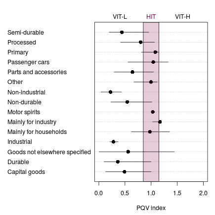
The next three figures summarize the distribution of the PQV index weighted by the value of trade, which shows the different types of TWT. When the PQV index equals one, the unit values of Chin𱏩D_bec.pngx0065;se exports and imports are equal. In the shaded area in the center—classified as HIT—export and import unit values are within approximately 30 percent of each other, which could plausibly indicate the exchange of similar goods at roughly similar prices and qualities. Because the largest share of TWT is in the VIT-L category, the PQV index will likely be concentrated in this zone. Most HS summary sections are, in fact, in the VIT-L zone as expected (figure 1). Animal products and at least parts of the distribution of edible fats and oils, pearls and precious metals, and wood and wood articles fall into the VIT-H zone, although they appear to be centered in the HIT zone. The arms and munitions section, where there was very little trade, had very low-priced exports compared to imports and an extremely small IQR. Cameras and instruments; hides, handbags, and luggage; and wood and wood articles had fairly broad IQRs, which likely indicate a wide variability in types of products and product quality within these sections.
Figure Note: Median and IQR weighted by value of total trade.
Medians of PQV index, as well as most of their IQRs, for broad economic categories are mainly in the VIT-L zone (figure 2). Export unit values relative to import unit values appear largest for the mainly-for-industry category, followed by primary goods, motor spirits, passenger cars, and other. Export unit values relative to import unit values are lowest for industrial and non-industrial goods, and these categories have small IQRs as well. Goods not elsewhere specified have a wide IQR, which might be expected for a catch-all category. However, the IQRs for capital goods, durable goods, mainly for households, parts and accessories, and passenger cars are also fairly wide, which may be surprising.
Figure Note: Median and IQR weighted by value of total trade.
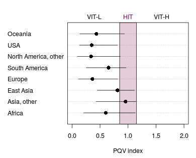
The PQV index is highest for China’s trade with other Asia and East Asia, which means Chinese export unit values are relatively higher than import unit values for these regions (figure 3). The index is lowest for its trade with Europe, other North America, and the USA, all of which are more developed regions. The index is in-between for China’s trade with Africa and South America.
Figure Note: Median and IQR weighted by value of total trade.
This section first examines factors that may determine whether an occurrence of Chinese trade is one way or two way. Explanatory variables mainly involve differences between countries as discussed in the section on explanations of OWT and TWT. Variables linked to trade costs, ownership types of trading Chinese firms, and different customs regimes are also included. The second part of this section examines the relationship between these same explanatory variables and the PQV index that is used to differentiate VIT-L, HIT, and VIT-H.
I create indexes to proxy for differences in endowments of labor and capital, skill level of the workforce, similar stage of development, country size, and trade costs. To capture the effects of differences in relative factor endowments between China and its trading partners, I use the absolute value of the log of country j’s annual capital-labor ratio minus the log of China’s annual capital labor ratio: . I use the difference between the annual average years of school for China and its trade partners to represent the difference in skill levels of the work force: . The absolute value of the differences in log per capita GDP at purchasing power parity is used to indicate whether China and its trade partners are at a similar stage of economic development: . Because some research suggests that TWT may arise from similarities in tastes shared by consumers in countries of a similar size instead of differences in factor endowments, i.e. the (Linder hypothesis), I construct an index to represent country size in a similar fashion as the absolute value of the differences in logs between China’s trade partners’ total GDP and its own GDP. Trade costs are the logs of the ratios of the cif value to the fob value between the destination and source countries. Data for these variables were constructed from sources specified in the section on data, and summary statistics for them are shown in the following table. The first four variables in the table vary over countries and over years, but are the same for all product categories. Trade costs vary over years and countries and products at the HS4 level.
| Variable | 1st quartile | Median | Mean | 3rd quartile |
| Capital-labor index | 0.559 | 1.286 | 1.405 | 2.155 |
| Labor skill index | -1.900 | 1.000 | 0.742 | 3.400 |
| Similarity index | 0.497 | 1.019 | 1.109 | 1.603 |
| Size index | 3.445 | 5.156 | 5.180 | 6.518 |
| Trade cost | 0.028 | 0.031 | 0.030 | 0.033 |
I create the continuous variables from sources described in the data section and merge them with the Chinese Customs data. The result is an unbalanced panel of 17,084,105 observations with 794,142 unique country-product combinations. Due to missing values, the merged data have 20 percent fewer observations than the OWT and TWT data used in the previous section (21,423,319 observations). I assume that the missing data are random and do not contain information that may affect the statistical results and maintain that, given the breadth of these data, valid inferences can be over the entire pattern of Chinese merchandise and agricultural trade for this period.
I construct other categorical variables for the model from the Chinese Customs data itself. Firm type is classified as state-owned firms (SOEs), joint ventures, foreign-invested firms, collectives, or private Chinese firms. Each ownership type is well represented with over a million observations; it is perhaps surprising to see the large number of observations linked to SOEs (table 8). Firm type varies over products and countries but is the only variable in the model that does not change over time. The variable for customs regime represents aggregates of either ordinary trade or processing trade. The customs data track several types of processing trade mainly depending upon which materials the foreign or domestic firms own; all these types are combined into one variable—processing trade. Firms that import under this regime have all tariffs rebated when they later export products using those imported inputs. Processing trade captures China’s role as a major assembler in global value chains in which China imports inputs, assembles them into other goods, and then exports them. Chinese processing trade began in the 1980s and grew to around a third of total imports and exports by the early 2000s, but has since declined as a share of total trade. For this 21 year period, processing trade averages a little less than a quarter of all trade. All non-processing trade was aggregated into the ordinary trade category except entrepôt trade was not used.
| Variable | Level | Count |
| Firm type | State-owned | 4,747,045 |
| Joint venture | 3,077,925 | |
| Foreign invested | 3,410,095 | |
| Collective | 1,690,832 | |
| Private Chinese | 4,158,208 | |
| Customs regime | Ordinary trade | 13,017,175 |
| Processing trade | 4,066,930 | |
| TWT, strict | No (0) | 14,233,166 |
| Yes (1) | 2,850,939 | |
| TWT(0.01) | No (0) | 15,113,922 |
| Yes (1) | 1,970,183 | |
The response variables are similarly categorical and indicate the presence or absence of TWT. As before, I use the strict definition (TWT, strict) and the one-percent definition, TWT(0.01), that counts trade as being two way only when the minimum flow is at least 1 percent of the maximum flow. Let represent the response variable and be equal to 1 if trade is two way and otherwise equal to 0. Next, I estimate a fixed effects logit model for these data to ascertain which factors increase the probability of observing TWT. This is represented mathematically as follows with the logistic cumulative distribution function on the right hand side:
| (6) |
where
are observations of explanatory variables
are product-country fixed effects and
is
the vector of parameters to be estimated.
The inclusion of fixed effects is important because the many traded products and numbers of countries involved will influence the type of trade. Omitting the fixed effects would likely result in considerable unaccounted for heterogeneity and biased results. Although fixed effects are important in this case, they complicate the approach considerably. Greene [12] shows that, although it is possible to estimate a reasonably large number of fixed-effects parameters by dummy variables, maximum likelihood estimation becomes increasingly biased as the number of individual effects increases, particularly when the time effects are small. Besides the issue of bias, the dummy variable approach is infeasible in this case, as there are over 700,000 fixed effects. Recently, Stammann, Heiss, and McFadden [21] have devised an approach to obtain the unconditional maximum likelihood estimates through an iterative demeaning procedure that removes the fixed effects, thus eliminating the bias from the large number of fixed effects. Their approach performs well in simulation studies and is feasible with large datasets.15
Despite the removal of the product-country fixed effects, a potential bias remains due to the time effects. Hahn and Newey [14] have proposed techniques to control for this type of bias in maximum likelihood estimation. I thus follow the Stammann-Heiss-McFadden approach with Hahn-Newey bias reduction to estimate the maximum likelihood equation.
For both the strict TWT and TWT(0.01) runs, the algorithm to remove the fixed effects converges in less than 10 iterations, and the likelihood ratio statistic shows that both models are statistically significant compared to the null model (table 9). Estimation of the bias for the time dimension also converged quickly. All of the parameter estimates with the bias correction are highly significant statistically except for trade cost in the TWT, strict run.
| Variable | TWT, strict | TWT(0.01) |
| Joint venture | -0.466*** | -0.310*** |
| (0.003) | (0.003) | |
| Foreign invested | 0.202*** | 0.267*** |
| (0.002) | (0.003) | |
| Collective | -2.268*** | -1.917*** |
| (0.004) | (0.005) | |
| Private Chinese | 0.095*** | -0.110*** |
| (0.002) | (0.003) | |
| Processing trade | -1.589*** | -1.152*** |
| (0.002) | (0.002) | |
| Trade cost | -0.801 | 1.433** |
| (0.491) | (0.536) | |
| Labor skill index | -0.170*** | -0.199*** |
| (0.003) | (0.003) | |
| Capital-labor index | 0.344*** | 0.216*** |
| (0.006) | (0.006) | |
| Similarity index | -1.098*** | -0.813*** |
| (0.009) | (0.010) | |
| Size index | 0.496*** | 0.416*** |
| (0.004) | (0.005) | |
| Observations | 17,084,105 | 17,084,105 |
| Fixed effects | 794,142 | 794,142 |
| Max. log likelihood | -4,298,571 | -3,618,846 |
| P-value likelihood ratio test | 2.22e-22 | 2.22e-22 |
Because the estimated coefficients are difficult to interpret directly, I compute the average partial effects . The partial effects are computed averaging over the fixed effects and also holding other variables at their means. Because the relationship between the response variable and independent variable is nonlinear, the effect could be different for other values of the variables that are held constant. For the most part, the correction for the time effects did not result in major changes in the average partial effects, and estimates in the TWT, strict run and the TWT(0.01) run are broadly similar (table 10).
SOEs are the reference level for firm types. Thus, in the corrected TWT(0.01) column, the partial effect of -0.038 for joint venture means that at average values of the data, a hypothetical export or import by a joint venture has a 0.038 lesser probability of being part of a TWT than a hypothetical trade by a SOE. In contrast, a hypothetical export or import by a foreign-invested firm has 0.0349 greater probability of being a TWT than that by a SOE. Collectives appear to engage relatively less in TWT (or participate more in OWT) than other firms. Although the sign changes between the two runs for private Chinese firms, both estimates are fairly small and imply that these firms have about the same probability of engaging in TWT as SOEs. Ordinary trade is the reference level for customs regime. The coefficient in the same column for processing trade implies that a trade by a processor has a probability of being part of a TWT that is 0.133 less than that of an ordinary trader at average values of the data. This is consistent of the view that processors import inputs under one HS code, employ capital and labor to transform those inputs into other products, and then export those products under different HS codes.
Average partial effects for continuous variables are instantaneous changes in the response variable given a small change in the explanatory variable while the other variables are held constant at their mean values. The estimate for trade cost, the only continuous variable whose sign changes between the two runs, is not statistically significant in the strict TWT run and positive (0.1848) in the other run, indicating that higher trade costs increase the probability of observing TWT as opposed to OWT. This result contradicts concepts and results in Bergstrand and Egger [4]. Fukao et al. [11] use distance as their indicator of trade costs and also find a negative relationship with TWT. The lack of variability in the statistically corrected cif-fob margins (see table 7) likely contributes to this result. In addition, Bergstrand and Egger do not include country fixed effects, which likely absorb some of the trade costs in this model.
| Strict TWT | Strict TWT | TWT(0.01) | TWT(0.01) | |
| Variable | Uncorrected | Corrected | Uncorrected | Corrected |
| Joint venture | -0.0571 | -0.0599 | -0.0359 | -0.0380 |
| Foreign invested | 0.0261 | 0.0275 | 0.0330 | 0.0349 |
| Collective | -0.2131 | -0.2206 | -0.1646 | -0.1720 |
| Private Chinese | 0.0123 | 0.0129 | -0.0131 | -0.0138 |
| Processing trade | -0.1830 | -0.1906 | -0.1262 | -0.1327 |
| Trade cost | -0.0983 | -0.1053 | 0.1761 | 0.1848 |
| Labor skill index | -0.0218 | -0.0228 | -0.0240 | -0.0254 |
| Capital-labor index | 0.0441 | 0.0463 | 0.0261 | 0.0276 |
| Similarity index | -0.1400 | -0.1472 | -0.0977 | -0.1034 |
| Size index | 0.0633 | 0.0665 | 0.0500 | 0.0529 |
The estimate for the capital-labor index, which is positive and statistically significant, implies that a larger difference in the capital-labor ratio increases the probability of China’s trade being two-way. This positive estimate runs counter to the negative result in Bergstrand and Egger and the literature that views TWT as resulting from specialization within industries and not requiring factor movements in the source or destination countries [15]. However, Fukao et al. [11] also find a positive relationship between differences in factor endowments and TWT in their case study of the electrical machinery industry, i.e. as the difference in factor endowments grows, the probability of TWT increases. Martín-Montaner and Orts [17] similarly find a positive relationship between differences in capital per worker and the proportion of Spain’s trade that is two-way. The results here and in these other studies call into question the way that differences in factor endowments affect the probability of TWT. Empirically both positive and negative estimates commonly occur. Nevertheless, the magnitude of the effect in this study is small (0.0276).
The results for the labor skill index and the similarity index are negative and imply that smaller differences in skill levels between China and its trade partners and more similar per capita income between China and its trade partners increase the probability of TWT. These results indicate that TWT is more likely to occur between countries with similarly skilled workforces and at similar levels of development than OWT. These results are consistent with those of Fukao et al. who find a significant negative relationship between differences in per capita income and TWT. Their result for education level is similarly negative but not statistically significant. In contrast, Martín-Montaner and Orts find a positive relationship between income differences and TWT, although their results for human capital differences and TWT are negative. Bergstrand and Egger do not include comparable variables.
In this subsection, I estimate a linear model to examine possible determinants of the PQV index using the subset of the data with TWT. Recall that higher values of this index indicate that China’s export unit values are relatively higher than its import unit values and that one interpretation is that higher unit values serve as a sign of higher quality and vice versa. The explanatory variables are the same ones used in the previous subsection. The PQV index varies between 0 and 2; I take its log, which extends its range close to zero and aids in interpretability.16
Before estimating the model, I compute the share of the total variation in the log of the PQV index that is due to the individual product-country effects and to the time effects and find that together these fixed effects account for half of the variation in the response variable. The variation in the log of the PQV index due to the product-country effects is 0.446, and the variation due to the time effects is 0.0580. Next, I estimate several versions of the following model.17
| (7) |
where
is the matrix of observations of explanatory variables
are product-country effects
are time effects
are idiosyncratic error terms and
is
the vector of parameters to be estimated.
First, I estimate the pooled model, which assumes that parameter values do not vary across products, countries, or years, or equivalently that and in equation 7 equal 0. All parameter estimates are highly significant, and the model as a whole is significant as indicated by the low value of the F-statistic p-value, but the is quite low, indicating that these variables explain little of the variation in the PQV index (table 11). As before, SOEs are the base level of firm types, and compared to them, TWT by foreign-invested firms have higher-valued exports than imports; the same is true for joint ventures but to a lesser extent. Relative to SOEs, private firms tend to have slightly higher valued exports than imports, while collectives tend to have slightly lower-valued exports than imports.
| Variable | Pooled | Fixed-I | Fixed-IT | Random |
| Joint venture | 0.196*** | — | — | 0.164*** |
| (0.003) | (0.003) | |||
| Foreign-invested | 0.346*** | — | — | 0.361*** |
| (0.003) | (0.003) | |||
| Collective | -0.062*** | — | — | -0.082*** |
| (0.006) | (0.005) | |||
| Private Chinese | 0.078*** | — | — | 0.038*** |
| (0.003) | (0.003) | |||
| Processing trade | 0.637*** | 0.408*** | 0.398*** | 0.428*** |
| (0.003) | (0.003) | (0.003) | (0.003) | |
| Capital-labor index | 0.108*** | 0.183*** | 0.009 | 0.158*** |
| (0.004) | (0.007) | (0.007) | (0.006) | |
| Similarity index | -0.064*** | 0.040*** | 0.102*** | -0.040*** |
| (0.005) | (0.011) | (0.014) | (0.008) | |
| Size index | -0.073*** | 0.049*** | 0.022*** | -0.048*** |
| (0.001) | (0.005) | (0.005) | (0.002) | |
| Labor skill index | -0.101*** | -0.0370** | -0.032*** | -0.082*** |
| (0.001) | (0.003) | (0.003) | (0.001) | |
| Trade cost | 7.805*** | 6.093*** | 0.425 | 3.566*** |
| (0.175) | (0.550) | (0.574) | 0.338 | |
| Constant | -9.147*** | — | — | -4.894*** |
| (0.180) | (0.348) | |||
| Observations | 1,948,736 | 1,948,736 | 1,948,736 | 1,948,736 |
| Fixed effects | 0 | 158364 | 158385 | — |
| 0.055 | 0.038 | 0.042 | 0.054 | |
| F-statistic p-value | 2.2e-16 | 2.2e-16 | 2.22e-16 | 2.22e-16 |
Given that product and country fixed effects account for a large share of the total variation in the response variable, it is unlikely that assumptions of the pooled model will hold. A test of the need for the individual effects strongly suggests that they should be in the model.18 Next, I estimate the model with individual fixed effects using the within transform, which sweeps out the fixed effects and variables that do not change over time (column “Fixed-I” in table 11). In addition, indications are that time effects are also needed.19 Column “Fixed-IT” in table 11 presents parameter estimates for a run that includes product, country, and time effects. A random effects model is more efficient than fixed effects and also produces estimates for the parameters that do not vary over time (column “Random”). The random effects’ estimates for the ownership types of firms in this column are fairly similar to the estimates for the pooled model. Unfortunately, the random effects model is inconsistent if the random effects are correlated with explanatory variables. A Hausman specification test for this possibility rejects the random effects model.20 All runs reported in table 11 are significant as a whole, as indicated by the F-statistic p-value, and have a number of statistically significant individual variables, but the low s show that these variables explain little of the variation in the response variable. From a purely statistical point of view, given the importance of the fixed efforts and problems with the pooled and random effects runs, the fixed-IT run appears best despite the fact that it has a couple of variables whose estimates are not statistically significant. Next, I discuss the estimates in this column.
The estimate for processing trade suggests that this type of customs regime has a PQV index that is 49 percent higher than that of ordinary trade, a fairly large difference.21 This implies that processing trade is associated with lower valued imports and higher valued exports.
The estimate for the capital-labor index is small and not statistically significant, which suggests that differences in the capital-labor ratio between China and its partners has little effect on the relative unit values of China’s exports and imports. The estimate for trade cost is not statistically significant either; the effects of trade costs could be absorbed by the product, country, and time fixed effects.
The significant positive result for the similarity index implies that, as the difference between China’s per capita income and that of its trade partners increases, China’s exports become higher priced relative to its imports, or conversely China’s exports to countries with more similar incomes are relatively lower valued. If we consider China trading mainly with Europe and North America, this result is surprising because the difference in per capita income between China and these regions is fairly large, and China appears to have specialized in lower valued exports to these regions. On the other hand, if China trades mainly with Africa, other Asia, and South America, where China’s per capita GDP is similar to or exceeds those of countries in these regions, the result is as expected. The estimate implies that a one-unit increase in this index would lead to an increase in the PQV index of around 10 percent.
The significant but small positive result for the size index implies that as China’s size (measured by total GDP) diverges from that of its trade partners, the PQV index becomes larger. The significant negative estimate for the labor skill index implies that as differences between China’s labor skill level and those of its trade partners increase, the PQV index decreases. This is consistent with the view that China’s exports to its more developed trade partners who have higher skilled workforces are priced relatively lower than its imports from those regions. Conversely, because the negative estimate implies that smaller differences between labor skill levels of China and its trade partners leads to a higher PQV index, it also supports the supposition that China’s exports are relatively higher priced to trade partners with more equally skilled workers.
This paper establishes that OWT consistently accounted for slightly less than three quarters of total Chinese trade between 1995 and 2015. During this period, China’s total volume of trade and numbers of products traded both rose substantially. The sectoral composition of China’s OWT changed. Exports of machines and electrical equipment greatly increased, but imports of these products declined. China’s textile trade continued to be significant, but its relative importance waned on both the export and import sides. There was an upsurge in China’s imports of mineral products, but its exports of these products weakened. China traded more with East Asia than with other regions; however, the relative importance of its East Asian trade has fallen, while the share with other Asian countries has risen. Processing trade, compared to ordinary trade, increases the probability of observing OWT. In addition, trade by collectives relative to other types of firms increase the probability of observing OWT.
China’s TWT is characterized by a growing share of VIT-L (relatively lower priced exports than imports). One interpretation of this result is that China has specialized in low quality exports based on similar qualitative divisions of labor. Not surprisingly, China’s trade in similarly priced products (HIT) is the smallest of its segments of TWT, although it is only slightly smaller than its VIT-H. China’s exports and imports of similar products are also fairly similarly priced when it trades with other Asian countries. However, its exports of similar products to the United States, other North America, and Europe are priced less than its imports from these regions. In addition, processing trade contributes more to higher valued exports than imports than ordinary trade. Among the types of firms, foreign-invested firms increase the likelihood of observing TWT the most and raise the PQV index the most.
This paper is among the few to examine the ability of indexes of differences among countries to explain the relative price of exports and imports in a country’s TWT. In the case of China between 1995 and 2015, greater differences in the stage of development, measured by per capita GDP, and in size, measured by total GDP, between China and its trade partners contributed to higher-priced Chinese exports relative to imports. In contrast, more similar labor skill levels, measured by years of school, contributed to higher priced Chinese exports relative to imports.
The likelihood of Chinese TWT increases when certain indexes indicate that China and its trade partners are more similar, but the reverse is true with other indexes. For example, both more similar per capita income and more similar workforce skill levels between China and its trade partners increase the probability of observing TWT. In contrast, greater differences in stage of development and in capital-labor ratios make Chinese TWT more likely.
As stated in the background section, some theoretical literature views TWT as occurring mainly between similar countries and as being more benign than OWT because it does not require readjustments of capital and labor in either of the trading countries. In this regard, empirical research has focused on the sign of the capital-labor ratio in estimations of the likelihood of TWT, and findings have varied. The previous theoretical work, such as Krugman’s often cited 1981 paper [16], was not presented as definitively explaining the relationship between TWT and factor movements but as presenting one possible explanation of facts observed at the time. This work and other empirical work show that the facts vary at different places and times. A future challenge will be to develop a more general understanding of the linkages between the types of trade and factor reallocations.
[1] Ando, Mitsuyo. “Fragmentation and Vertical Intra-industry Trade in East Asia.” The North American Journal of Economics and Finance 17, iss. 3 (December 2006): 257–281.
[2] Azhar, Abdul K. and Robert J.R. Elliott. “On the Measurement of Product Quality in Intra-Industry Trade.” Review of World Economics 142, iss. 3 (October 2006): 476–495.
[3] Baltagi, Badi. Econometric Analysis of Panel Data, 4th ed. Chichester: Wiley & Sons, 2008.
[4] Bergstrand, Jeffrey H. and Peter Egger. “Trade Costs and Intra-Industry Trade.” Review of World Economics 142, iss. 3 (October 2006): 433–458.
[5] Croissant, Yves and Giovanni Millo. “Panel Data Econometrics in R: The plm Package.” Journal of Statistical Software 27, iss. 2 (2008). https://www.jstatsoft.org/article/view/v027i02
[6] Davis, Donald R. “Intra-industry trade: A Heckscher-Ohlin-Ricardo approach.” Journal of International Economics 39, iss. 34 (November 1995): 201–226.
[7] Egger, Hartmut Peter Egger, David Greenaway. “Intra-industry Trade with Multinational Firms.” European Economic Review 51, iss. 8 (November 2007): 1959–1984.
[8] Falvey, Rodney E. “Commercial Policy and Intra-industry Trade”, Journal of International Economics 11, iss. 4 (1981): 495–511.
[9] Falvey, Rodney E., and Henryk Kierzkowski. “Product Quality, Intra-industry Trade and (Im)perfect Competition.” In Protection and Competition in International Trade: Essays in Honor of W.M. Corden, 143–161, Oxford: Blackwell, 1987.
[10] Fontagné, Lionel and Michael Freudenberg. “Intra-Industry Trade: Methodological Issues Reconsidered.” CEPII Working Paper no. 1997-01, January 1997.
[11] Fukao,Kyoji, Hikari Ishido, and Keiko Ito. “Vertical Intra-industry Trade and Foreign Direct Investment in East Asia.” Journal of the Japanese and International Economies 17, iss. 4 (December 2003): 468–506.
[12] Greene, William. “The Behaviour of the Maximum Likelihood Estimator of Limited Dependent Variable Models in the Presence of Fixed Effects.” Econometrics Journal 7, iss. 3 (2004): 98–119.
[13] Grubel, Herbert G. and Peter J. Lloyd. Intra-industry Trade: The Theory and Measurement of International Trade in Differentiated Products, New York, Wiley, 1975.
[14] Hahn, Jinyong and Whitney Newey. “Jackknife and Analytical Bias Reduction for Nonlinear Panel Models.” Econometrica 72, iss. 4 (2004): 1295–1319.
[15] Helpman, Elhanan and Paul R. Krugman. Market Structure and Foreign Trade. Cambridge: MIT Press, 1985.
[16] Krugman, Paul R. “Intraindustry Specialization and the Gains from Trade.” Journal of Political Economy 89, no. 5 (1981): 959–973.
[17] Martín-Montaner, Joan A. and Vicente Orts Ríos. “Vertical Specialization and Intra-industry Trade: The Role of Factor Endowments.” Weltwirtschaftliches Archiv 138, no. 2 (2002): 340–365.
[18] R Core Team. R: A Language and Environment for Statistical Computing. Vienna: R Foundation for Statistical Computing, 2017.
[19] Abd-el-Rahman, Kamal. “Firms’ Competitive and National Comparative Advantages as Joint Determinants of Trade Composition.” Review of World Economics 127, no. 1 (1991): 83–97.
[20] Sawyer, William C., Richard L. Sprinkle, Kiril Tochkov, “Patterns and Determinants of Intra-industry Trade in Asia.” Journal of Asian Economics 21, iss. 5 (October 2010): 485–493.
[21] Stammann, Amrei, Florian Heiss, and Daniel McFadden. “Estimation of Fixed Effects Logit Models with Large Panel Data.” Beitrge zur Jahrestagung des Vereins fr Socialpolitik 2016: Demographischer Wandel-Session: Microeconometrics, Working Paper No. G01-V3, August 2016.
[22] Stammann, Amrei, Daniel Czarnowske, and Florian Heiss. “bife: Binary Choice Models with Fixed Effects .” R Package version 0.2: March 2017.
[23] Xing,Yuqing. “Foreign Direct Investment and China’s Bilateral Intra-industry Trade with Japan and the US.” Journal of Asian Economics 18, iss. 4 (August 2007): 685–700.
[24] Zhang, Yansheng, Dawei Li, Changyong Yang, and Qiong Du. “On the Value Chain and International Specialization of China’s Pharmaceutical Industry.” USITC Journal of International Commerce and Economics 3, no. 1, (May 2011): 81–107.
[25] Zheng, Yingmei, and Jianhong Qi. “Empirical Analysis of the Structure of Sino-US Agricultural Trade.” China & World Economy 15, no. 4 (2007): 35–51.
1Calculated from the China Statistical Yearbook, 2016, http://www.stats.gov.cn/tjsj/ndsj/2016/indexeh.htm.
2This is somewhat similar to the Linder hypothesis that countries with similar demand structures trade more with each other.
3Falvey [8] and Falvey and Kierzkowski [9] have spurred an enormous amount of empirical work but not very much theoretical work.
4These approaches are more comprehensive than only reporting Grubel-Lloyd indexes but are highly correlated with it. I also present Grubel-Lloyd indexes as a reference point.
5Azhar and Elliott [2] delineate other desirable properties of this index.
6A table in the next section show actual numbers by year.
7For this I use the HS 2002 classification by section. https://unstats.un.org/unsd/tradekb/Knowledgebase/50043/HS-2002-Classification-by-Section
8I use the concordance provided by the fifth revision of the UN Statistical Commission in 2016. https://unstats.un.org/unsd/tradekb/Knowledgebase/50671/5th-revision-of-the-Classification-by-Broad-Economic-Categories-BEC “Classification by Broad Economic Categories” by the department of Economic and Social Affairs of the UN provides a complete general introduction to BECs.
9The concordance proceeded reasonably well but not without some difficulties. Some Pacific islands did not match. In some cases parts of a country were counted as separate countries in the Chinese data. For example, Ceuta and Melilla appear as separate countries in the Chinese data, I include them with Spain.
10Zhang et al. [24] report that discrepancies could occur because countries disagree where to classify certain products under the HS code. Reporting under the HS system is believed to be fairly accurate, but inadvertent errors and corruption by customs officials also lead to discrepancies.
11http://oecdinsights.org/2016/11/02/statistical-insights-new-oecd-database-on-international-transport-and-insurance-costs/
12The growth rate is the annual rate of change in nominal trade. Inflation was low for most of this period, and these annual figures are believed to approximate the change in real trade reasonably well.
13Small values of the IQR indicate little dispersion in the data and vice versa. The IQR is the distance between the 75th percentile and the 25th percentile (the middle half of the data).
14Semi-durable refers to a consumer category of goods that have an expected lifetime of more than one year but less than three years.
15Chamberlain devised a method in 1980 to condition out the fixed effects and then estimate the conditional log likelihood function; this approach is implemented in Stata’s clogit package and elsewhere [3]. The Stammann, Heiss, McFadden approach yields numerically identical estimates in small and moderately sized datasets, and importantly produces estimates in large datasets, when the Chamberlain approach chokes and does not solve. I use the R [18] package “bife” by Stammann et al. [22].
16The minimum PQV value is 3.57e-7 whose log is -14.8, so there is no danger that the index may reach negative infinity.
17These estimates and related calculations were made using the plm package in R [5].
18An F-test rejects the hypothesis that the with a value of 8.79 with 158,360 and 1,790,400 degrees of freedom.
19An F-test that the yields a value of 421.8, which is firmly rejected with 20 and 1,790,300 degrees of freedom.
20The Hausman chi-square statistic is 9228 with 10 degrees of freedom, firmly rejecting the consistency of the random effects model.
21The interpretation of a dummy variable d that switches form 0 to 1 in a semilog model is that percent change in the response variable is given by .