ECONOMICS WORKING PAPER SERIES


WHENCE THE BEEF?:
THE EFFECT OF REPEALING MANDATORY COUNTRY OF ORIGIN LABELING (COOL) USING A VERTICALLY INTEGRATED ARMINGTON MODEL WITH MONTE CARLO SIMULATION


Ross J. Hallren
Alexandra Opanasets


Working Paper 2016-9-A


U.S. INTERNATIONAL TRADE COMMISSION

500 E Street SW

Washington, DC 20436

September 2016


Office of Economics working papers are the result of ongoing professional research of USITC Staff and are solely meant to represent the opinions and professional research of individual authors. These papers are not meant to represent in any way the views of the U.S. International Trade Commission or any of its individual Commissioners. Working papers are circulated to promote the active exchange of ideas between USITC Staff and recognized experts outside the USITC and to promote professional development of Office Staff by encouraging outside professional critique of staff research.

Whence the Beef?: The Effect of Repealing Mandatory Country of Origin Labeling (COOL) using a Vertically Integrated Armington Model with Monte Carlo Simulation

Ross J. Hallren and Alexandra Opanasets

Office of Economics Working Paper 2016-09-A

September 2016


ABSTRACT


Increasingly, international trade policy analysis explores the economic effects of changes in ad-valorem tariffs, or ad-valorem equivalent non-tariff measures, on vertically integrated markets for which high quality data are not available. Standard Constant Elasticity of Substitution (CES) Armington models fail to account for either vertical linkages or parameter uncertainty. Here we introduce a modified Armington CES vertically integrated two-sector model, with nested Armington Elasticities, that incorporates uncertainty in the estimates of Armington Elasticities and market shares through a Monte Carlo simulation. As an illustrative case, we model the effects of changes in country of origin labeling (COOL) rules on the market shares of domestic and foreign cattle in the U.S. beef market. By accounting for parameter uncertainty in this way, we are able to illustrate the distribution of potential effects of repealing mandatory COOL. Moreover, we are able to decompose the effect of repealing COOL via its effect on relative prices, information available to consumers, and the quasi-general equilibrium effect. Finally, we uncover the conditions under which Canada and Mexico would benefit from the repeal of mandatory COOL by at least as much as they claim in their WTO filings against the regulation.


Ross Hallren

Office of Economics

Ross.Hallren@usitc.gov


Alexandra Opanasets

Office of Economics and NYU Shanghai


Overview

One of the great challenges of economic policy analysis is incorporating uncertainty into model estimates. A common practice in analyzing international trade policy changes is to utilize estimates from industry level studies when parameterizing the Armington Constant Elasticity of Substitution (CES) partial equilibrium (PE) model. Additionally, one must obtain information on production quantities and market shares for all countries under consideration. These data are then treated as if they are known with certainty. However, in many cases, we estimate the effects of policies on very narrow markets for which even import and production data are collected with some error. We propose incorporating a series of simple Monte Carlo simulations to account for uncertainty in the Armington CES PE model’s parameter values and production information. Doing so allows the user to generate a distribution of possible economic effects given uncertainty in the information on model inputs. Ultimately, this allows the economist to produce estimates that are more robust to parameterization and more illustrative of the range of possible effects.

Additionally, even in the world of PE modelling, where we focus on narrow markets and try to capture the most direct effects of policy changes, economists often want to analyze markets with strong vertical linkages. Failing to account for these linkages, which the standard Armington (1969) model does, might cause us to produce estimates of the economic impact of the potential policy change that are higher or lower than the true impact. Moreover, by not accounting for these linkages, we miss the broader multi-market dynamics of the effect of the policy.

As an illustrative case, we construct a vertically integrated, nested CES Armington PE model that predicts the effect on market shares of a change in labelling requirement for cattle imported into the U.S. from Canada and Mexico. We contribute to the country of origin labeling (COOL) literature by explicitly modeling vertical linkages between production stages. Additionally, we decompose the effect of the repeal of COOL through the change in relative prices (i.e. the Armington effect), the quasi-general equilibrium market expansion effect, and the change in information available to consumers (i.e. the information effect). Finally, we allow for uncertainty in parameter estimates and conduct sensitivity analysis through Monte Carlo simulation.

This case is timely because Congress amended rules on Country of Origin Labeling (COOL) in the 2016 Consolidated Appropriations Act. As of 2016, mandatory country of origin labeling is no longer required for muscle cuts of beef and pork imported into the U.S. Previously, Congress had applied a COOL requirement on producers that imported cattle from Mexico and Canada and processed the animals in domestic feedlots or slaughterhouses. The repeal of this labeling requirement represents a decline in a trade cost, for beef imports from NAFTA countries, that is easily converted into a tariff equivalent.

Additionally, the relaxation of country-specific labeling requirements reduces the amount of information available to consumers at purchase and thus affects how consumers and producers think about imports vis-à-vis the domestic variety. From the consumer perspective, they will be less aware of the difference between foreign and domestic varieties after the rule change, so we would expect the rule change to affect the Armington elasticity by increasing the willingness to substitute between foreign and domestic varieties of a given product as well as between two foreign varieties. This suggests that we should consider modeling the rule change not only as an import tariff equivalent reduction on NAFTA beef imports but also as a positive shock on the willingness to substitute between foreign and domestic varieties and across foreign varieties. We are able to decompose the effect of repealing COOL via its effect on relative prices, information available to consumers, and the quasi-general equilibrium market expansion effect.

The paper proceeds as follows. First, we derive the market share equations for our model and incorporate Monte Carlo simulation. We then introduce our COOL case study, present our results, and conclude.

Derivation of Market Share Equations

The Armington (1969) CES model is standard in the economics literature and easy to use and customize. As figure 1 shows, the model assumes customers (consumers or firms) choose between an array of goods from a sector of interest offered by domestic (U.S.) or foreign suppliers (F). Consumers are willing to substitute between foreign and domestic units at a constant rate, where the elasticity of substitution is (α).[1] The model works for any value of α. However, we would expect the elasticity to have a value greater than one since in this case a fall in the price of good j, ceteris paribus, improves its competitiveness and thus its market share.[2]

We might think it unrealistic to assume that consumers are willing to substitute between foreign and domestic goods at the same rate that they would substitute between two units from different foreign countries. In figure 2, we divide the foreign branch of the tree into Canada and Mexico branches. Here α is the foreign-domestic elasticity of substitution and β is the intra-foreign elasticity of substitution. Therefore, we have nested a second branch within our original tree, such that feedlot companies that choose to stock their facilities with foreign calves may also choose the import country of origin.

Finally, because the U.S. cattle industry is a vertically structured, multi-sector industry and the change in labelling requirements could affect the upstream and downstream asymmetrically or generate feedback loops, we change our conceptual framework to the one pictured in figure 3. Here we have feedlots that buy calves from farms and then sell mature cattle to slaughterhouses. We allow for a nested CES structure at both the upstream and the downstream stages.

Here we provide technical details for expanding the standard one-sector Armington (1969) CES PE model to a vertical, multi-sector nested CES model. While we specifically derive a two-sector, two nest CES model, the technique described here can be generalized to any number of nests and any number of vertically linked sectors. Moreover, we account for parameter uncertainty via Monte Carlo simulation.

In our applications, we directly observe initial market shares. We calculate the ad-valorem equivalent of the proposed policy change and simulate the elasticities of substitution via Monte Carlo simulation. While we do not observe prices, we normalize them to one and use shift parameters calibrated to initial, observed market shares. We will derive a three country model: the domestic market (U.S.), Canada, and Mexico. A three country model is sufficient because Canada and Mexico are de-facto the U.S.’s only trading partners in the live cattle market. Although we only use three countries here, we could easily extend the model to any number of countries.

In the basic Armington CES model (figure 1), the market share for good j from country c is a function of its price relative to the price of good j from all countries, taste parameters, and the elasticity of substitution. We can modify the standard result from Armington (1969) and derive simple equations for the market shares for domestic and foreign calves in U.S. feedlots[3]. These equations are

S U , FU = γ U P U , FU 1α γ U P U , FU 1α + γ F P F , FU 1α = φ 1 MathType@MTEF@5@5@+= feaagKart1ev2aqatCvAUfeBSjuyZL2yd9gzLbvyNv2CaerbuLwBLn hiov2DGi1BTfMBaeXatLxBI9gBaerbd9wDYLwzYbItLDharqqtubsr 4rNCHbGeaGqiVCI8FfYJH8YrFfeuY=Hhbbf9v8qqaqFr0xc9pk0xbb a9q8WqFfeaY=biLkVcLq=JHqpepeea0=as0Fb9pgeaYRXxe9vr0=vr 0=vqpWqaaeaabiGaciaacaqabeaadaqaaqaaaOqaaabaaaaaaaaape Gaae4ua8aadaWgaaWcbaWdbiaabwfaa8aabeaak8qacaGGSaWdamaa BaaaleaapeGaaeOraiaabwfaa8aabeaak8qacqGH9aqpdaWcaaWdae aapeGaeq4SdC2damaaBaaaleaapeGaamyvaaWdaeqaaOWdbiaadcfa paWaaSbaaSqaa8qacaWGvbaapaqabaGcpeGaaiila8aadaqhaaWcba WdbiaadAeacaWGvbaapaqaa8qacaaIXaGaeyOeI0IaeqySdegaaaGc paqaa8qacqaHZoWzpaWaaSbaaSqaa8qacaWGvbaapaqabaGcpeGaam iua8aadaWgaaWcbaWdbiaadwfaa8aabeaak8qacaGGSaWdamaaDaaa leaapeGaamOraiaadwfaa8aabaWdbiaaigdacqGHsislcqaHXoqyaa GccqGHRaWkcqaHZoWzpaWaaSbaaSqaa8qacaWGgbaapaqabaGcpeGa amiua8aadaWgaaWcbaWdbiaadAeaa8aabeaak8qacaGGSaWdamaaDa aaleaapeGaamOraiaadwfaa8aabaWdbiaaigdacqGHsislcqaHXoqy aaaaaOGaeyypa0JaeqOXdO2damaaBaaaleaapeGaaGymaaWdaeqaaa aa@625E@      (1)

S F , FU = γ F P F , FU 1α γ U P U , FU 1α + γ F P F , FU 1α = φ 2 MathType@MTEF@5@5@+= feaagKart1ev2aqatCvAUfeBSjuyZL2yd9gzLbvyNv2CaerbuLwBLn hiov2DGi1BTfMBaeXatLxBI9gBaerbd9wDYLwzYbItLDharqqtubsr 4rNCHbGeaGqiVCI8FfYJH8YrFfeuY=Hhbbf9v8qqaqFr0xc9pk0xbb a9q8WqFfeaY=biLkVcLq=JHqpepeea0=as0Fb9pgeaYRXxe9vr0=vr 0=vqpWqaaeaabiGaciaacaqabeaadaqaaqaaaOqaaabaaaaaaaaape Gaae4ua8aadaWgaaWcbaWdbiaabAeaa8aabeaak8qacaGGSaWdamaa BaaaleaapeGaaeOraiaabwfaa8aabeaak8qacqGH9aqpdaWcaaWdae aapeGaeq4SdC2damaaBaaaleaapeGaamOraaWdaeqaaOWdbiaadcfa paWaaSbaaSqaa8qacaWGgbaapaqabaGcpeGaaiila8aadaqhaaWcba WdbiaadAeacaWGvbaapaqaa8qacaaIXaGaeyOeI0IaeqySdegaaaGc paqaa8qacqaHZoWzpaWaaSbaaSqaa8qacaWGvbaapaqabaGcpeGaam iua8aadaWgaaWcbaWdbiaadwfaa8aabeaak8qacaGGSaWdamaaDaaa leaapeGaamOraiaadwfaa8aabaWdbiaaigdacqGHsislcqaHXoqyaa GccqGHRaWkcqaHZoWzpaWaaSbaaSqaa8qacaWGgbaapaqabaGcpeGa amiua8aadaWgaaWcbaWdbiaadAeaa8aabeaak8qacaGGSaWdamaaDa aaleaapeGaamOraiaadwfaa8aabaWdbiaaigdacqGHsislcqaHXoqy aaaaaOGaeyypa0JaeqOXdO2damaaBaaaleaapeGaaGOmaaWdaeqaaa aa@6232@      (2)

The market shares sum to one, and the shift parameters ( γ U , γ F MathType@MTEF@5@5@+= feaagKart1ev2aqatCvAUfeBSjuyZL2yd9gzLbvyNv2CaerbuLwBLn hiov2DGi1BTfMBaeXatLxBI9gBaerbd9wDYLwzYbItLDharqqtubsr 4rNCHbGeaGqiVCI8FfYJH8YrFfeuY=Hhbbf9v8qqaqFr0xc9pk0xbb a9q8WqFfeaY=biLkVcLq=JHqpepeea0=as0Fb9pgeaYRXxe9vr0=vr 0=vqpWqaaeaabiGaciaacaqabeaadaqaaqaaaOqaaabaaaaaaaaape Gaeq4SdC2damaaBaaaleaapeGaamyvaaWdaeqaaOWdbiaacYcacqaH ZoWzpaWaaSbaaSqaa8qacaWGgbaapaqabaaaaa@3C7D@  ) also sum to one.

φ 1 + φ 2 =1 MathType@MTEF@5@5@+= feaagKart1ev2aqatCvAUfeBSjuyZL2yd9gzLbvyNv2CaerbuLwBLn hiov2DGi1BTfMBaeXatLxBI9gBaerbd9wDYLwzYbItLDharqqtubsr 4rNCHbGeaGqiVCI8FfYJH8YrFfeuY=Hhbbf9v8qqaqFr0xc9pk0xbb a9q8WqFfeaY=biLkVcLq=JHqpepeea0=as0Fb9pgeaYRXxe9vr0=vr 0=vqpWqaaeaabiGaciaacaqabeaadaqaaqaaaOqaaabaaaaaaaaape GaeqOXdO2damaaBaaaleaapeGaaGymaaWdaeqaaOWdbiabgUcaRiab eA8aQ9aadaWgaaWcbaWdbiaaikdaa8aabeaak8qacqGH9aqpcaaIXa aaaa@3E88@      (3)
γ U + γ F =1 MathType@MTEF@5@5@+= feaagKart1ev2aqatCvAUfeBSjuyZL2yd9gzLbvyNv2CaerbuLwBLn hiov2DGi1BTfMBaeXatLxBI9gBaerbd9wDYLwzYbItLDharqqtubsr 4rNCHbGeaGqiVCI8FfYJH8YrFfeuY=Hhbbf9v8qqaqFr0xc9pk0xbb a9q8WqFfeaY=biLkVcLq=JHqpepeea0=as0Fb9pgeaYRXxe9vr0=vr 0=vqpWqaaeaabiGaciaacaqabeaadaqaaqaaaOqaaabaaaaaaaaape Gaeq4SdC2damaaBaaaleaapeGaamyvaaWdaeqaaOWdbiabgUcaRiab eo7aN9aadaWgaaWcbaWdbiaadAeaa8aabeaak8qacqGH9aqpcaaIXa aaaa@3E8A@     (4)

To incorporate different rates of substitution between domestic and foreign units and across foreign varieties (see figure 2), we replace P F MathType@MTEF@5@5@+= feaagKart1ev2aqatCvAUfeBSjuyZL2yd9gzLbvyNv2CaerbuLwBLn hiov2DGi1BTfMBaeXatLxBI9gBaerbd9wDYLwzYbItLDharqqtubsr 4rNCHbGeaGqiVCI8FfYJH8YrFfeuY=Hhbbf9v8qqaqFr0xc9pk0xbb a9q8WqFfeaY=biLkVcLq=JHqpepeea0=as0Fb9pgeaYRXxe9vr0=vr 0=vqpWqaaeaabiGaciaacaqabeaadaqaaqaaaOqaaabaaaaaaaaape Gaamiua8aadaWgaaWcbaWdbiaadAeaa8aabeaaaaa@3806@  with a price index that incorporates the prices from Canada and Mexico.[4] The procedure would be the same if U.S. feedlots imported from more foreign countries: we would add the prices for each of these import countries into the index.  

P F , FU = ( ρ C P C , FU 1β + ρ M P M , FU 1β ) 1 1β MathType@MTEF@5@5@+= feaagKart1ev2aqatCvAUfeBSjuyZL2yd9gzLbvyNv2CaerbuLwBLn hiov2DGi1BTfMBaeXatLxBI9gBaerbd9wDYLwzYbItLDharqqtubsr 4rNCHbGeaGqiVCI8FfYJH8YrFfeuY=Hhbbf9v8qqaqFr0xc9pk0xbb a9q8WqFfeaY=biLkVcLq=JHqpepeea0=as0Fb9pgeaYRXxe9vr0=vr 0=vqpWqaaeaabiGaciaacaqabeaadaqaaqaaaOqaaabaaaaaaaaape Gaamiua8aadaWgaaWcbaWdbiaadAeaa8aabeaak8qacaGGSaWdamaa BaaaleaapeGaamOraiaadwfaa8aabeaak8qacqGH9aqpdaqadaWdae aapeGaeqyWdi3damaaBaaaleaapeGaam4qaaWdaeqaaOWdbiaadcfa paWaaSbaaSqaa8qacaWGdbaapaqabaGcpeGaaiila8aadaqhaaWcba WdbiaadAeacaWGvbaapaqaa8qacaaIXaGaeyOeI0IaeqOSdigaaOGa ey4kaSIaeqyWdi3damaaBaaaleaapeGaamytaaWdaeqaaOWdbiaadc fapaWaaSbaaSqaa8qacaWGnbaapaqabaGcpeGaaiila8aadaqhaaWc baWdbiaadAeacaWGvbaapaqaa8qacaaIXaGaeyOeI0IaeqOSdigaaa GccaGLOaGaayzkaaWdamaaCaaaleqabaWdbmaalaaapaqaa8qacaaI Xaaapaqaa8qacaaIXaGaeyOeI0IaeqOSdigaaaaaaaa@596B@      (5)

where
ρ C + ρ M =1 MathType@MTEF@5@5@+= feaagKart1ev2aqatCvAUfeBSjuyZL2yd9gzLbvyNv2CaerbuLwBLn hiov2DGi1BTfMBaeXatLxBI9gBaerbd9wDYLwzYbItLDharqqtubsr 4rNCHbGeaGqiVCI8FfYJH8YrFfeuY=Hhbbf9v8qqaqFr0xc9pk0xbb a9q8WqFfeaY=biLkVcLq=JHqpepeea0=as0Fb9pgeaYRXxe9vr0=vr 0=vqpWqaaeaabiGaciaacaqabeaadaqaaqaaaOqaaabaaaaaaaaape GaeqyWdi3damaaBaaaleaapeGaam4qaaWdaeqaaOWdbiabgUcaRiab eg8aY9aadaWgaaWcbaWdbiaad2eaa8aabeaak8qacqGH9aqpcaaIXa aaaa@3EB1@      (6)

We calculate the value shares of Canadian and Mexican calves in U.S. feedlots as

S C , FU = S F , FU * S C , F , FU MathType@MTEF@5@5@+= feaagKart1ev2aqatCvAUfeBSjuyZL2yd9gzLbvyNv2CaerbuLwBLn hiov2DGi1BTfMBaeXatLxBI9gBaerbd9wDYLwzYbItLDharqqtubsr 4rNCHbGeaGqiVCI8FfYJH8YrFfeuY=Hhbbf9v8qqaqFr0xc9pk0xbb a9q8WqFfeaY=biLkVcLq=JHqpepeea0=as0Fb9pgeaYRXxe9vr0=vr 0=vqpWqaaeaabiGaciaacaqabeaadaqaaqaaaOqaaabaaaaaaaaape Gaam4ua8aadaWgaaWcbaWdbiaadoeaa8aabeaak8qacaGGSaWdamaa BaaaleaapeGaamOraiaadwfaa8aabeaak8qacqGH9aqpcaWGtbWdam aaBaaaleaapeGaamOraaWdaeqaaOWdbiaacYcapaWaaSbaaSqaa8qa caWGgbGaamyvaaWdaeqaaOWdbiaacQcacaWGtbWdamaaBaaaleaape Gaam4qaaWdaeqaaOWdbiaacYcapaWaaSbaaSqaa8qacaWGgbaapaqa baGcpeGaaiila8aadaWgaaWcbaWdbiaadAeacaWGvbaapaqabaaaaa@482F@      (7)

S C , FU =[ γ F P F , FU 1α γ U P U , FU 1α + γ F P F , FU 1α ][ ρ C P C , FU 1β ρ C P C , FU 1β + ρ M P M , FU 1β ]= φ 3 MathType@MTEF@5@5@+= feaagKart1ev2aqatCvAUfeBSjuyZL2yd9gzLbvyNv2CaerbuLwBLn hiov2DGi1BTfMBaeXatLxBI9gBaerbd9wDYLwzYbItLDharqqtubsr 4rNCHbGeaGqiVCI8FfYJH8YrFfeuY=Hhbbf9v8qqaqFr0xc9pk0xbb a9q8WqFfeaY=biLkVcLq=JHqpepeea0=as0Fb9pgeaYRXxe9vr0=vr 0=vqpWqaaeaabiGaciaacaqabeaadaqaaqaaaOqaaabaaaaaaaaape Gaam4ua8aadaWgaaWcbaWdbiaadoeaa8aabeaak8qacaGGSaWdamaa BaaaleaapeGaamOraiaadwfaa8aabeaak8qacqGH9aqpdaWadaWdae aapeWaaSaaa8aabaWdbiabeo7aN9aadaWgaaWcbaWdbiaadAeaa8aa beaak8qacaWGqbWdamaaBaaaleaapeGaamOraaWdaeqaaOWdbiaacY capaWaa0baaSqaa8qacaWGgbGaamyvaaWdaeaapeGaaGymaiabgkHi Tiabeg7aHbaaaOWdaeaapeGaeq4SdC2damaaBaaaleaapeGaamyvaa WdaeqaaOWdbiaadcfapaWaaSbaaSqaa8qacaWGvbaapaqabaGcpeGa aiila8aadaqhaaWcbaWdbiaadAeacaWGvbaapaqaa8qacaaIXaGaey OeI0IaeqySdegaaOGaey4kaSIaeq4SdC2damaaBaaaleaapeGaamOr aaWdaeqaaOWdbiaadcfapaWaaSbaaSqaa8qacaWGgbaapaqabaGcpe Gaaiila8aadaqhaaWcbaWdbiaadAeacaWGvbaapaqaa8qacaaIXaGa eyOeI0IaeqySdegaaaaaaOGaay5waiaaw2faamaadmaapaqaa8qada WcaaWdaeaapeGaeqyWdi3damaaBaaaleaapeGaam4qaaWdaeqaaOWd biaadcfapaWaaSbaaSqaa8qacaWGdbaapaqabaGcpeGaaiila8aada qhaaWcbaWdbiaadAeacaWGvbaapaqaa8qacaaIXaGaeyOeI0IaeqOS digaaaGcpaqaa8qacqaHbpGCpaWaaSbaaSqaa8qacaWGdbaapaqaba GcpeGaamiua8aadaWgaaWcbaWdbiaadoeaa8aabeaak8qacaGGSaWd amaaDaaaleaapeGaamOraiaadwfaa8aabaWdbiaaigdacqGHsislcq aHYoGyaaGccqGHRaWkcqaHbpGCpaWaaSbaaSqaa8qacaWGnbaapaqa baGcpeGaamiua8aadaWgaaWcbaWdbiaad2eaa8aabeaak8qacaGGSa WdamaaDaaaleaapeGaamOraiaadwfaa8aabaWdbiaaigdacqGHsisl cqaHYoGyaaaaaaGccaGLBbGaayzxaaGaeyypa0JaeqOXdO2damaaBa aaleaapeGaaG4maaWdaeqaaaaa@88FE@      (8)

S M , FU = S F , FU * S M , F , FU MathType@MTEF@5@5@+= feaagKart1ev2aqatCvAUfeBSjuyZL2yd9gzLbvyNv2CaerbuLwBLn hiov2DGi1BTfMBaeXatLxBI9gBaerbd9wDYLwzYbItLDharqqtubsr 4rNCHbGeaGqiVCI8FfYJH8YrFfeuY=Hhbbf9v8qqaqFr0xc9pk0xbb a9q8WqFfeaY=biLkVcLq=JHqpepeea0=as0Fb9pgeaYRXxe9vr0=vr 0=vqpWqaaeaabiGaciaacaqabeaadaqaaqaaaOqaaabaaaaaaaaape Gaam4ua8aadaWgaaWcbaWdbiaad2eaa8aabeaak8qacaGGSaWdamaa BaaaleaapeGaamOraiaadwfaa8aabeaak8qacqGH9aqpcaWGtbWdam aaBaaaleaapeGaamOraaWdaeqaaOWdbiaacYcapaWaaSbaaSqaa8qa caWGgbGaamyvaaWdaeqaaOWdbiaacQcacaWGtbWdamaaBaaaleaape GaamytaaWdaeqaaOWdbiaacYcapaWaaSbaaSqaa8qacaWGgbaapaqa baGcpeGaaiila8aadaWgaaWcbaWdbiaadAeacaWGvbaapaqabaaaaa@4843@      (9)

S M , FU =[ γ F P F , FU 1α γ U P U , FU 1α + γ F P F , FU 1α ][ ρ M P M , FU 1β ρ C P C , FU 1β + ρ M P M , FU 1β ]= φ 4 MathType@MTEF@5@5@+= feaagKart1ev2aqatCvAUfeBSjuyZL2yd9gzLbvyNv2CaerbuLwBLn hiov2DGi1BTfMBaeXatLxBI9gBaerbd9wDYLwzYbItLDharqqtubsr 4rNCHbGeaGqiVCI8FfYJH8YrFfeuY=Hhbbf9v8qqaqFr0xc9pk0xbb a9q8WqFfeaY=biLkVcLq=JHqpepeea0=as0Fb9pgeaYRXxe9vr0=vr 0=vqpWqaaeaabiGaciaacaqabeaadaqaaqaaaOqaaabaaaaaaaaape Gaam4ua8aadaWgaaWcbaWdbiaad2eaa8aabeaak8qacaGGSaWdamaa BaaaleaapeGaamOraiaadwfaa8aabeaak8qacqGH9aqpdaWadaWdae aapeWaaSaaa8aabaWdbiabeo7aN9aadaWgaaWcbaWdbiaadAeaa8aa beaak8qacaWGqbWdamaaBaaaleaapeGaamOraaWdaeqaaOWdbiaacY capaWaa0baaSqaa8qacaWGgbGaamyvaaWdaeaapeGaaGymaiabgkHi Tiabeg7aHbaaaOWdaeaapeGaeq4SdC2damaaBaaaleaapeGaamyvaa WdaeqaaOWdbiaadcfapaWaaSbaaSqaa8qacaWGvbaapaqabaGcpeGa aiila8aadaqhaaWcbaWdbiaadAeacaWGvbaapaqaa8qacaaIXaGaey OeI0IaeqySdegaaOGaey4kaSIaeq4SdC2damaaBaaaleaapeGaamOr aaWdaeqaaOWdbiaadcfapaWaaSbaaSqaa8qacaWGgbaapaqabaGcpe Gaaiila8aadaqhaaWcbaWdbiaadAeacaWGvbaapaqaa8qacaaIXaGa eyOeI0IaeqySdegaaaaaaOGaay5waiaaw2faamaadmaapaqaa8qada WcaaWdaeaapeGaeqyWdi3damaaBaaaleaapeGaamytaaWdaeqaaOWd biaadcfapaWaaSbaaSqaa8qacaWGnbaapaqabaGcpeGaaiila8aada qhaaWcbaWdbiaadAeacaWGvbaapaqaa8qacaaIXaGaeyOeI0IaeqOS digaaaGcpaqaa8qacqaHbpGCpaWaaSbaaSqaa8qacaWGdbaapaqaba GcpeGaamiua8aadaWgaaWcbaWdbiaadoeaa8aabeaak8qacaGGSaWd amaaDaaaleaapeGaamOraiaadwfaa8aabaWdbiaaigdacqGHsislcq aHYoGyaaGccqGHRaWkcqaHbpGCpaWaaSbaaSqaa8qacaWGnbaapaqa baGcpeGaamiua8aadaWgaaWcbaWdbiaad2eaa8aabeaak8qacaGGSa WdamaaDaaaleaapeGaamOraiaadwfaa8aabaWdbiaaigdacqGHsisl cqaHYoGyaaaaaaGccaGLBbGaayzxaaGaeyypa0JaeqOXdO2damaaBa aaleaapeGaaGinaaWdaeqaaaaa@891D@      (10)

where

φ 2 = φ 3 + φ 4 MathType@MTEF@5@5@+= feaagKart1ev2aqatCvAUfeBSjuyZL2yd9gzLbvyNv2CaerbuLwBLn hiov2DGi1BTfMBaeXatLxBI9gBaerbd9wDYLwzYbItLDharqqtubsr 4rNCHbGeaGqiVCI8FfYJH8YrFfeuY=Hhbbf9v8qqaqFr0xc9pk0xbb a9q8WqFfeaY=biLkVcLq=JHqpepeea0=as0Fb9pgeaYRXxe9vr0=vr 0=vqpWqaaeaabiGaciaacaqabeaadaqaaqaaaOqaaabaaaaaaaaape GaeqOXdO2damaaBaaaleaapeGaaGOmaaWdaeqaaOWdbiabg2da9iab eA8aQ9aadaWgaaWcbaWdbiaaiodaa8aabeaak8qacqGHRaWkcqaHgp GApaWaaSbaaSqaa8qacaaI0aaapaqabaaaaa@40A4@      (11)

The shift parameters ( γ U , γ F , ρ U , ρ f MathType@MTEF@5@5@+= feaagKart1ev2aqatCvAUfeBSjuyZL2yd9gzLbvyNv2CaerbuLwBLn hiov2DGi1BTfMBaeXatLxBI9gBaerbd9wDYLwzYbItLDharqqtubsr 4rNCHbGeaGqiVCI8FfYJH8YrFfeuY=Hhbbf9v8qqaqFr0xc9pk0xbb a9q8WqFfeaY=biLkVcLq=JHqpepeea0=as0Fb9pgeaYRXxe9vr0=vr 0=vqpWqaaeaabiGaciaacaqabeaadaqaaqaaaOqaaabaaaaaaaaape Gaeq4SdC2damaaBaaaleaapeGaamyvaaWdaeqaaOWdbiaacYcacqaH ZoWzpaWaaSbaaSqaa8qacaWGgbaapaqabaGcpeGaaiilaiabeg8aY9 aadaWgaaWcbaWdbiaadwfaa8aabeaak8qacaGGSaGaeqyWdi3damaa BaaaleaapeGaamOzaaWdaeqaaaaa@440A@  ) are necessary because we may not be able to observe the prices paid by U.S. feedlots but only the market shares of U.S., Canada, and Mexico’s calves purchased by U.S. feedlots. With this flexibility, we do not need prices, which are exogenous in the model. Consequently, we normalize all prices to one and calibrate the shift parameters such that, when all prices are one, the initial calculated market share values match the actual observed market shares. To calculate ρ M MathType@MTEF@5@5@+= feaagKart1ev2aqatCvAUfeBSjuyZL2yd9gzLbvyNv2CaerbuLwBLn hiov2DGi1BTfMBaeXatLxBI9gBaerbd9wDYLwzYbItLDharqqtubsr 4rNCHbGeaGqiVCI8FfYJH8YrFfeuY=Hhbbf9v8qqaqFr0xc9pk0xbb a9q8WqFfeaY=biLkVcLq=JHqpepeea0=as0Fb9pgeaYRXxe9vr0=vr 0=vqpWqaaeaabiGaciaacaqabeaadaqaaqaaaOqaaabaaaaaaaaape GaeqyWdi3damaaBaaaleaapeGaamytaaWdaeqaaaaa@38F8@  we substitute equation (10) into equation (8), rearrange terms, and use (6). Once we solve for ρ M MathType@MTEF@5@5@+= feaagKart1ev2aqatCvAUfeBSjuyZL2yd9gzLbvyNv2CaerbuLwBLn hiov2DGi1BTfMBaeXatLxBI9gBaerbd9wDYLwzYbItLDharqqtubsr 4rNCHbGeaGqiVCI8FfYJH8YrFfeuY=Hhbbf9v8qqaqFr0xc9pk0xbb a9q8WqFfeaY=biLkVcLq=JHqpepeea0=as0Fb9pgeaYRXxe9vr0=vr 0=vqpWqaaeaabiGaciaacaqabeaadaqaaqaaaOqaaabaaaaaaaaape GaeqyWdi3damaaBaaaleaapeGaamytaaWdaeqaaaaa@38F8@ , we calculate ρ C MathType@MTEF@5@5@+= feaagKart1ev2aqatCvAUfeBSjuyZL2yd9gzLbvyNv2CaerbuLwBLn hiov2DGi1BTfMBaeXatLxBI9gBaerbd9wDYLwzYbItLDharqqtubsr 4rNCHbGeaGqiVCI8FfYJH8YrFfeuY=Hhbbf9v8qqaqFr0xc9pk0xbb a9q8WqFfeaY=biLkVcLq=JHqpepeea0=as0Fb9pgeaYRXxe9vr0=vr 0=vqpWqaaeaabiGaciaacaqabeaadaqaaqaaaOqaaabaaaaaaaaape GaeqyWdi3damaaBaaaleaapeGaam4qaaWdaeqaaaaa@38EE@  using equation (6) again. Thus, those shift parameters are

ρ M = φ 4 P C , FU 1β φ 3 P M , FU 1β + φ 4 P C , FU 1β MathType@MTEF@5@5@+= feaagKart1ev2aqatCvAUfeBSjuyZL2yd9gzLbvyNv2CaerbuLwBLn hiov2DGi1BTfMBaeXatLxBI9gBaerbd9wDYLwzYbItLDharqqtubsr 4rNCHbGeaGqiVCI8FfYJH8YrFfeuY=Hhbbf9v8qqaqFr0xc9pk0xbb a9q8WqFfeaY=biLkVcLq=JHqpepeea0=as0Fb9pgeaYRXxe9vr0=vr 0=vqpWqaaeaabiGaciaacaqabeaadaqaaqaaaOqaaabaaaaaaaaape GaeqyWdi3damaaBaaaleaapeGaamytaaWdaeqaaOWdbiabg2da9maa laaapaqaa8qacqaHgpGApaWaaSbaaSqaa8qacaaI0aaapaqabaGcpe Gaamiua8aadaWgaaWcbaWdbiaadoeaa8aabeaak8qacaGGSaWdamaa DaaaleaapeGaamOraiaadwfaa8aabaWdbiaaigdacqGHsislcqaHYo Gyaaaak8aabaWdbiabeA8aQ9aadaWgaaWcbaWdbiaaiodaa8aabeaa k8qacaWGqbWdamaaBaaaleaapeGaamytaaWdaeqaaOWdbiaacYcapa Waa0baaSqaa8qacaWGgbGaamyvaaWdaeaapeGaaGymaiabgkHiTiab ek7aIbaakiabgUcaRiabeA8aQ9aadaWgaaWcbaWdbiaaisdaa8aabe aak8qacaWGqbWdamaaBaaaleaapeGaam4qaaWdaeqaaOWdbiaacYca paWaa0baaSqaa8qacaWGgbGaamyvaaWdaeaapeGaaGymaiabgkHiTi abek7aIbaaaaaaaa@5C80@      (12)

ρ C = φ 3 P M , FU 1β φ 3 P M , FU 1β + φ 4 P C , FU 1β MathType@MTEF@5@5@+= feaagKart1ev2aqatCvAUfeBSjuyZL2yd9gzLbvyNv2CaerbuLwBLn hiov2DGi1BTfMBaeXatLxBI9gBaerbd9wDYLwzYbItLDharqqtubsr 4rNCHbGeaGqiVCI8FfYJH8YrFfeuY=Hhbbf9v8qqaqFr0xc9pk0xbb a9q8WqFfeaY=biLkVcLq=JHqpepeea0=as0Fb9pgeaYRXxe9vr0=vr 0=vqpWqaaeaabiGaciaacaqabeaadaqaaqaaaOqaaabaaaaaaaaape GaeqyWdi3damaaBaaaleaapeGaam4qaaWdaeqaaOWdbiabg2da9maa laaapaqaa8qacqaHgpGApaWaaSbaaSqaa8qacaaIZaaapaqabaGcpe Gaamiua8aadaWgaaWcbaWdbiaad2eaa8aabeaak8qacaGGSaWdamaa DaaaleaapeGaamOraiaadwfaa8aabaWdbiaaigdacqGHsislcqaHYo Gyaaaak8aabaWdbiabeA8aQ9aadaWgaaWcbaWdbiaaiodaa8aabeaa k8qacaWGqbWdamaaBaaaleaapeGaamytaaWdaeqaaOWdbiaacYcapa Waa0baaSqaa8qacaWGgbGaamyvaaWdaeaapeGaaGymaiabgkHiTiab ek7aIbaakiabgUcaRiabeA8aQ9aadaWgaaWcbaWdbiaaisdaa8aabe aak8qacaWGqbWdamaaBaaaleaapeGaam4qaaWdaeqaaOWdbiaacYca paWaa0baaSqaa8qacaWGgbGaamyvaaWdaeaapeGaaGymaiabgkHiTi abek7aIbaaaaaaaa@5C7F@      (13)

To calculate γ U MathType@MTEF@5@5@+= feaagKart1ev2aqatCvAUfeBSjuyZL2yd9gzLbvyNv2CaerbuLwBLn hiov2DGi1BTfMBaeXatLxBI9gBaerbd9wDYLwzYbItLDharqqtubsr 4rNCHbGeaGqiVCI8FfYJH8YrFfeuY=Hhbbf9v8qqaqFr0xc9pk0xbb a9q8WqFfeaY=biLkVcLq=JHqpepeea0=as0Fb9pgeaYRXxe9vr0=vr 0=vqpWqaaeaabiGaciaacaqabeaadaqaaqaaaOqaaabaaaaaaaaape Gaeq4SdC2damaaBaaaleaapeGaamyvaaWdaeqaaaaa@38E7@  we substitute equation (2) into equation (1), rearrange terms and use (4). Once we solve for γ U MathType@MTEF@5@5@+= feaagKart1ev2aqatCvAUfeBSjuyZL2yd9gzLbvyNv2CaerbuLwBLn hiov2DGi1BTfMBaeXatLxBI9gBaerbd9wDYLwzYbItLDharqqtubsr 4rNCHbGeaGqiVCI8FfYJH8YrFfeuY=Hhbbf9v8qqaqFr0xc9pk0xbb a9q8WqFfeaY=biLkVcLq=JHqpepeea0=as0Fb9pgeaYRXxe9vr0=vr 0=vqpWqaaeaabiGaciaacaqabeaadaqaaqaaaOqaaabaaaaaaaaape Gaeq4SdC2damaaBaaaleaapeGaamyvaaWdaeqaaaaa@38E7@ , we calculate γ F MathType@MTEF@5@5@+= feaagKart1ev2aqatCvAUfeBSjuyZL2yd9gzLbvyNv2CaerbuLwBLn hiov2DGi1BTfMBaeXatLxBI9gBaerbd9wDYLwzYbItLDharqqtubsr 4rNCHbGeaGqiVCI8FfYJH8YrFfeuY=Hhbbf9v8qqaqFr0xc9pk0xbb a9q8WqFfeaY=biLkVcLq=JHqpepeea0=as0Fb9pgeaYRXxe9vr0=vr 0=vqpWqaaeaabiGaciaacaqabeaadaqaaqaaaOqaaabaaaaaaaaape Gaeq4SdC2damaaBaaaleaapeGaamOraaWdaeqaaaaa@38D8@  using equation (4) again. The resulting equations are

γ U = φ 1 P F , FU 1α φ 1 P F , FU 1α + φ 2 P U , FU 1α MathType@MTEF@5@5@+= feaagKart1ev2aqatCvAUfeBSjuyZL2yd9gzLbvyNv2CaerbuLwBLn hiov2DGi1BTfMBaeXatLxBI9gBaerbd9wDYLwzYbItLDharqqtubsr 4rNCHbGeaGqiVCI8FfYJH8YrFfeuY=Hhbbf9v8qqaqFr0xc9pk0xbb a9q8WqFfeaY=biLkVcLq=JHqpepeea0=as0Fb9pgeaYRXxe9vr0=vr 0=vqpWqaaeaabiGaciaacaqabeaadaqaaqaaaOqaaabaaaaaaaaape Gaeq4SdC2damaaBaaaleaapeGaamyvaaWdaeqaaOWdbiabg2da9maa laaapaqaa8qacqaHgpGApaWaaSbaaSqaa8qacaaIXaaapaqabaGcpe Gaamiua8aadaWgaaWcbaWdbiaadAeaa8aabeaak8qacaGGSaWdamaa DaaaleaapeGaamOraiaadwfaa8aabaWdbiaaigdacqGHsislcqaHXo qyaaaak8aabaWdbiabeA8aQ9aadaWgaaWcbaWdbiaaigdaa8aabeaa k8qacaWGqbWdamaaBaaaleaapeGaamOraaWdaeqaaOWdbiaacYcapa Waa0baaSqaa8qacaWGgbGaamyvaaWdaeaapeGaaGymaiabgkHiTiab eg7aHbaakiabgUcaRiabeA8aQ9aadaWgaaWcbaWdbiaaikdaa8aabe aak8qacaWGqbWdamaaBaaaleaapeGaamyvaaWdaeqaaOWdbiaacYca paWaa0baaSqaa8qacaWGgbGaamyvaaWdaeaapeGaaGymaiabgkHiTi abeg7aHbaaaaaaaa@5C70@      (14)

γ F = φ 2 P U , FU 1α φ 1 P F , FU 1α + φ 2 P U , FU 1α MathType@MTEF@5@5@+= feaagKart1ev2aqatCvAUfeBSjuyZL2yd9gzLbvyNv2CaerbuLwBLn hiov2DGi1BTfMBaeXatLxBI9gBaerbd9wDYLwzYbItLDharqqtubsr 4rNCHbGeaGqiVCI8FfYJH8YrFfeuY=Hhbbf9v8qqaqFr0xc9pk0xbb a9q8WqFfeaY=biLkVcLq=JHqpepeea0=as0Fb9pgeaYRXxe9vr0=vr 0=vqpWqaaeaabiGaciaacaqabeaadaqaaqaaaOqaaabaaaaaaaaape Gaeq4SdC2damaaBaaaleaapeGaamOraaWdaeqaaOWdbiabg2da9maa laaapaqaa8qacqaHgpGApaWaaSbaaSqaa8qacaaIYaaapaqabaGcpe Gaamiua8aadaWgaaWcbaWdbiaadwfaa8aabeaak8qacaGGSaWdamaa DaaaleaapeGaamOraiaadwfaa8aabaWdbiaaigdacqGHsislcqaHXo qyaaaak8aabaWdbiabeA8aQ9aadaWgaaWcbaWdbiaaigdaa8aabeaa k8qacaWGqbWdamaaBaaaleaapeGaamOraaWdaeqaaOWdbiaacYcapa Waa0baaSqaa8qacaWGgbGaamyvaaWdaeaapeGaaGymaiabgkHiTiab eg7aHbaakiabgUcaRiabeA8aQ9aadaWgaaWcbaWdbiaaikdaa8aabe aak8qacaWGqbWdamaaBaaaleaapeGaamyvaaWdaeqaaOWdbiaacYca paWaa0baaSqaa8qacaWGgbGaamyvaaWdaeaapeGaaGymaiabgkHiTi abeg7aHbaaaaaaaa@5C71@      (15)

In the downstream market, slaughterhouses, the market shares for slaughter animals from US feedlots and foreign feedlots are

S U , SU = δ U P U , SU 1σ δ U P U , SU 1σ + δ F P F , SU 1σ = φ 5 MathType@MTEF@5@5@+= feaagKart1ev2aqatCvAUfeBSjuyZL2yd9gzLbvyNv2CaerbuLwBLn hiov2DGi1BTfMBaeXatLxBI9gBaerbd9wDYLwzYbItLDharqqtubsr 4rNCHbGeaGqiVCI8FfYJH8YrFfeuY=Hhbbf9v8qqaqFr0xc9pk0xbb a9q8WqFfeaY=biLkVcLq=JHqpepeea0=as0Fb9pgeaYRXxe9vr0=vr 0=vqpWqaaeaabiGaciaacaqabeaadaqaaqaaaOqaaabaaaaaaaaape Gaam4ua8aadaWgaaWcbaWdbiaadwfaa8aabeaak8qacaGGSaWdamaa BaaaleaapeGaam4uaiaadwfaa8aabeaak8qacqGH9aqpdaWcaaWdae aapeGaeqiTdq2damaaBaaaleaapeGaamyvaaWdaeqaaOWdbiaadcfa paWaaSbaaSqaa8qacaWGvbaapaqabaGcpeGaaiila8aadaqhaaWcba WdbiaadofacaWGvbaapaqaa8qacaaIXaGaeyOeI0Iaeq4WdmhaaaGc paqaa8qacqaH0oazpaWaaSbaaSqaa8qacaWGvbaapaqabaGcpeGaam iua8aadaWgaaWcbaWdbiaadwfaa8aabeaak8qacaGGSaWdamaaDaaa leaapeGaam4uaiaadwfaa8aabaWdbiaaigdacqGHsislcqaHdpWCaa GccqGHRaWkcqaH0oazpaWaaSbaaSqaa8qacaWGgbaapaqabaGcpeGa amiua8aadaWgaaWcbaWdbiaadAeaa8aabeaak8qacaGGSaWdamaaDa aaleaapeGaam4uaiaadwfaa8aabaWdbiaaigdacqGHsislcqaHdpWC aaaaaOGaeyypa0JaeqOXdO2damaaBaaaleaapeGaaGynaaWdaeqaaa aa@6304@      (16)

S F , SU = δ F P F , SU 1σ δ U P U , SU 1σ + δ F P F , SU 1σ = φ 6 MathType@MTEF@5@5@+= feaagKart1ev2aqatCvAUfeBSjuyZL2yd9gzLbvyNv2CaerbuLwBLn hiov2DGi1BTfMBaeXatLxBI9gBaerbd9wDYLwzYbItLDharqqtubsr 4rNCHbGeaGqiVCI8FfYJH8YrFfeuY=Hhbbf9v8qqaqFr0xc9pk0xbb a9q8WqFfeaY=biLkVcLq=JHqpepeea0=as0Fb9pgeaYRXxe9vr0=vr 0=vqpWqaaeaabiGaciaacaqabeaadaqaaqaaaOqaaabaaaaaaaaape Gaam4ua8aadaWgaaWcbaWdbiaadAeaa8aabeaak8qacaGGSaWdamaa BaaaleaapeGaam4uaiaadwfaa8aabeaak8qacqGH9aqpdaWcaaWdae aapeGaeqiTdq2damaaBaaaleaapeGaamOraaWdaeqaaOWdbiaadcfa paWaaSbaaSqaa8qacaWGgbaapaqabaGcpeGaaiila8aadaqhaaWcba WdbiaadofacaWGvbaapaqaa8qacaaIXaGaeyOeI0Iaeq4WdmhaaaGc paqaa8qacqaH0oazpaWaaSbaaSqaa8qacaWGvbaapaqabaGcpeGaam iua8aadaWgaaWcbaWdbiaadwfaa8aabeaak8qacaGGSaWdamaaDaaa leaapeGaam4uaiaadwfaa8aabaWdbiaaigdacqGHsislcqaHdpWCaa GccqGHRaWkcqaH0oazpaWaaSbaaSqaa8qacaWGgbaapaqabaGcpeGa amiua8aadaWgaaWcbaWdbiaadAeaa8aabeaak8qacaGGSaWdamaaDa aaleaapeGaam4uaiaadwfaa8aabaWdbiaaigdacqGHsislcqaHdpWC aaaaaOGaeyypa0JaeqOXdO2damaaBaaaleaapeGaaGOnaaWdaeqaaa aa@62D8@      (17)

where

S U , SU + S F , SU =1 MathType@MTEF@5@5@+= feaagKart1ev2aqatCvAUfeBSjuyZL2yd9gzLbvyNv2CaerbuLwBLn hiov2DGi1BTfMBaeXatLxBI9gBaerbd9wDYLwzYbItLDharqqtubsr 4rNCHbGeaGqiVCI8FfYJH8YrFfeuY=Hhbbf9v8qqaqFr0xc9pk0xbb a9q8WqFfeaY=biLkVcLq=JHqpepeea0=as0Fb9pgeaYRXxe9vr0=vr 0=vqpWqaaeaabiGaciaacaqabeaadaqaaqaaaOqaaabaaaaaaaaape Gaam4ua8aadaWgaaWcbaWdbiaadwfaa8aabeaak8qacaGGSaWdamaa BaaaleaapeGaam4uaiaadwfaa8aabeaak8qacqGHRaWkcaWGtbWdam aaBaaaleaapeGaamOraaWdaeqaaOWdbiaacYcapaWaaSbaaSqaa8qa caWGtbGaamyvaaWdaeqaaOWdbiabg2da9iaaigdaaaa@4298@      (18)

Again, to incorporate the nested CES function we change the foreign price to a price index, where the shift parameters (θ’s) sum to one.

P F , SU = [ θ C P C , SU 1ϑ + θ M P M , SU 1ϑ ] 1 1ϑ MathType@MTEF@5@5@+= feaagKart1ev2aqatCvAUfeBSjuyZL2yd9gzLbvyNv2CaerbuLwBLn hiov2DGi1BTfMBaeXatLxBI9gBaerbd9wDYLwzYbItLDharqqtubsr 4rNCHbGeaGqiVCI8FfYJH8YrFfeuY=Hhbbf9v8qqaqFr0xc9pk0xbb a9q8WqFfeaY=biLkVcLq=JHqpepeea0=as0Fb9pgeaYRXxe9vr0=vr 0=vqpWqaaeaabiGaciaacaqabeaadaqaaqaaaOqaaabaaaaaaaaape Gaamiua8aadaWgaaWcbaWdbiaadAeaa8aabeaak8qacaGGSaWdamaa BaaaleaapeGaam4uaiaadwfaa8aabeaak8qacqGH9aqpdaWadaWdae aapeGaeqiUde3damaaBaaaleaapeGaam4qaaWdaeqaaOWdbiaadcfa paWaaSbaaSqaa8qacaWGdbaapaqabaGcpeGaaiila8aadaqhaaWcba WdbiaadofacaWGvbaapaqaa8qacaaIXaGaeyOeI0Iaeqy0dOeaaOGa ey4kaSIaeqiUde3damaaBaaaleaapeGaamytaaWdaeqaaOWdbiaadc fapaWaaSbaaSqaa8qacaWGnbaapaqabaGcpeGaaiila8aadaqhaaWc baWdbiaadofacaWGvbaapaqaa8qacaaIXaGaeyOeI0Iaeqy0dOeaaa GccaGLBbGaayzxaaWdamaaCaaaleqabaWdbmaalaaapaqaa8qacaaI Xaaapaqaa8qacaaIXaGaeyOeI0Iaeqy0dOeaaaaaaaa@59FC@      (19)

θ C + θ M =1 MathType@MTEF@5@5@+= feaagKart1ev2aqatCvAUfeBSjuyZL2yd9gzLbvyNv2CaerbuLwBLn hiov2DGi1BTfMBaeXatLxBI9gBaerbd9wDYLwzYbItLDharqqtubsr 4rNCHbGeaGqiVCI8FfYJH8YrFfeuY=Hhbbf9v8qqaqFr0xc9pk0xbb a9q8WqFfeaY=biLkVcLq=JHqpepeea0=as0Fb9pgeaYRXxe9vr0=vr 0=vqpWqaaeaabiGaciaacaqabeaadaqaaqaaaOqaaabaaaaaaaaape GaeqiUde3damaaBaaaleaapeGaam4qaaWdaeqaaOWdbiabgUcaRiab eI7aX9aadaWgaaWcbaWdbiaad2eaa8aabeaak8qacqGH9aqpcaaIXa aaaa@3E9D@      (20)

The domestic price for slaughter animals from U.S. feedlots is itself an index of prices paid for calves from domestic and foreign farms.

P U , SU = [ γ U P U , FU 1α + γ F P F , FU 1α ] 1 1α MathType@MTEF@5@5@+= feaagKart1ev2aqatCvAUfeBSjuyZL2yd9gzLbvyNv2CaerbuLwBLn hiov2DGi1BTfMBaeXatLxBI9gBaerbd9wDYLwzYbItLDharqqtubsr 4rNCHbGeaGqiVCI8FfYJH8YrFfeuY=Hhbbf9v8qqaqFr0xc9pk0xbb a9q8WqFfeaY=biLkVcLq=JHqpepeea0=as0Fb9pgeaYRXxe9vr0=vr 0=vqpWqaaeaabiGaciaacaqabeaadaqaaqaaaOqaaabaaaaaaaaape Gaamiua8aadaWgaaWcbaWdbiaadwfaa8aabeaak8qacaGGSaWdamaa BaaaleaapeGaam4uaiaadwfaa8aabeaak8qacqGH9aqpdaWadaWdae aapeGaeq4SdC2damaaBaaaleaapeGaamyvaaWdaeqaaOWdbiaadcfa paWaaSbaaSqaa8qacaWGvbaapaqabaGcpeGaaiila8aadaqhaaWcba WdbiaadAeacaWGvbaapaqaa8qacaaIXaGaeyOeI0IaeqySdegaaOGa ey4kaSIaeq4SdC2damaaBaaaleaapeGaamOraaWdaeqaaOWdbiaadc fapaWaaSbaaSqaa8qacaWGgbaapaqabaGcpeGaaiila8aadaqhaaWc baWdbiaadAeacaWGvbaapaqaa8qacaaIXaGaeyOeI0IaeqySdegaaa GccaGLBbGaayzxaaWdamaaCaaaleqabaWdbmaalaaapaqaa8qacaaI Xaaapaqaa8qacaaIXaGaeyOeI0IaeqySdegaaaaaaaa@59CE@      (21)

δ U + δ F =1 MathType@MTEF@5@5@+= feaagKart1ev2aqatCvAUfeBSjuyZL2yd9gzLbvyNv2CaerbuLwBLn hiov2DGi1BTfMBaeXatLxBI9gBaerbd9wDYLwzYbItLDharqqtubsr 4rNCHbGeaGqiVCI8FfYJH8YrFfeuY=Hhbbf9v8qqaqFr0xc9pk0xbb a9q8WqFfeaY=biLkVcLq=JHqpepeea0=as0Fb9pgeaYRXxe9vr0=vr 0=vqpWqaaeaabiGaciaacaqabeaadaqaaqaaaOqaaabaaaaaaaaape GaeqiTdq2damaaBaaaleaapeGaamyvaaWdaeqaaOWdbiabgUcaRiab es7aK9aadaWgaaWcbaWdbiaadAeaa8aabeaak8qacqGH9aqpcaaIXa aaaa@3E86@      (22)

We calculate the market shares for Canadian and Mexican slaughter animals as

S C , SU = S F , SU * S C , F , SU MathType@MTEF@5@5@+= feaagKart1ev2aqatCvAUfeBSjuyZL2yd9gzLbvyNv2CaerbuLwBLn hiov2DGi1BTfMBaeXatLxBI9gBaerbd9wDYLwzYbItLDharqqtubsr 4rNCHbGeaGqiVCI8FfYJH8YrFfeuY=Hhbbf9v8qqaqFr0xc9pk0xbb a9q8WqFfeaY=biLkVcLq=JHqpepeea0=as0Fb9pgeaYRXxe9vr0=vr 0=vqpWqaaeaabiGaciaacaqabeaadaqaaqaaaOqaaabaaaaaaaaape Gaam4ua8aadaWgaaWcbaWdbiaadoeaa8aabeaak8qacaGGSaWdamaa BaaaleaapeGaam4uaiaadwfaa8aabeaak8qacqGH9aqpcaWGtbWdam aaBaaaleaapeGaamOraaWdaeqaaOWdbiaacYcapaWaaSbaaSqaa8qa caWGtbGaamyvaaWdaeqaaOWdbiaacQcacaWGtbWdamaaBaaaleaape Gaam4qaaWdaeqaaOWdbiaacYcapaWaaSbaaSqaa8qacaWGgbaapaqa baGcpeGaaiila8aadaWgaaWcbaWdbiaadofacaWGvbaapaqabaaaaa@4856@      (23)

S C , F , SU =[ δ F P F , SU 1σ δ U P U , SU 1σ + δ F P F , SU 1σ ][ θ C P C , SU 1ϑ θ C P C , SU 1ϑ + θ M P M , SU 1ϑ ]= φ 7 MathType@MTEF@5@5@+= feaagKart1ev2aqatCvAUfeBSjuyZL2yd9gzLbvyNv2CaerbuLwBLn hiov2DGi1BTfMBaeXatLxBI9gBaerbd9wDYLwzYbItLDharqqtubsr 4rNCHbGeaGqiVCI8FfYJH8YrFfeuY=Hhbbf9v8qqaqFr0xc9pk0xbb a9q8WqFfeaY=biLkVcLq=JHqpepeea0=as0Fb9pgeaYRXxe9vr0=vr 0=vqpWqaaeaabiGaciaacaqabeaadaqaaqaaaOqaaabaaaaaaaaape Gaam4ua8aadaWgaaWcbaWdbiaadoeaa8aabeaak8qacaGGSaWdamaa BaaaleaapeGaamOraaWdaeqaaOWdbiaacYcapaWaaSbaaSqaa8qaca WGtbGaamyvaaWdaeqaaOWdbiabg2da9maadmaapaqaa8qadaWcaaWd aeaapeGaeqiTdq2damaaBaaaleaapeGaamOraaWdaeqaaOWdbiaadc fapaWaaSbaaSqaa8qacaWGgbaapaqabaGcpeGaaiila8aadaqhaaWc baWdbiaadofacaWGvbaapaqaa8qacaaIXaGaeyOeI0Iaeq4Wdmhaaa Gcpaqaa8qacqaH0oazpaWaaSbaaSqaa8qacaWGvbaapaqabaGcpeGa amiua8aadaWgaaWcbaWdbiaadwfaa8aabeaak8qacaGGSaWdamaaDa aaleaapeGaam4uaiaadwfaa8aabaWdbiaaigdacqGHsislcqaHdpWC aaGccqGHRaWkcqaH0oazpaWaaSbaaSqaa8qacaWGgbaapaqabaGcpe Gaamiua8aadaWgaaWcbaWdbiaadAeaa8aabeaak8qacaGGSaWdamaa DaaaleaapeGaam4uaiaadwfaa8aabaWdbiaaigdacqGHsislcqaHdp WCaaaaaaGccaGLBbGaayzxaaWaamWaa8aabaWdbmaalaaapaqaa8qa cqaH4oqCpaWaaSbaaSqaa8qacaWGdbaapaqabaGcpeGaamiua8aada WgaaWcbaWdbiaadoeaa8aabeaak8qacaGGSaWdamaaDaaaleaapeGa am4uaiaadwfaa8aabaWdbiaaigdacqGHsislcqaHrpGsaaaak8aaba WdbiabeI7aX9aadaWgaaWcbaWdbiaadoeaa8aabeaak8qacaWGqbWd amaaBaaaleaapeGaam4qaaWdaeqaaOWdbiaacYcapaWaa0baaSqaa8 qacaWGtbGaamyvaaWdaeaapeGaaGymaiabgkHiTiabeg9akbaakiab gUcaRiabeI7aX9aadaWgaaWcbaWdbiaad2eaa8aabeaak8qacaWGqb WdamaaBaaaleaapeGaamytaaWdaeqaaOWdbiaacYcapaWaa0baaSqa a8qacaWGtbGaamyvaaWdaeaapeGaaGymaiabgkHiTiabeg9akbaaaa aakiaawUfacaGLDbaacqGH9aqpcqaHgpGApaWaaSbaaSqaa8qacaaI 3aaapaqabaaaaa@8BA9@     (24)

S M , SU = S F , SU * S M , F , SU MathType@MTEF@5@5@+= feaagKart1ev2aqatCvAUfeBSjuyZL2yd9gzLbvyNv2CaerbuLwBLn hiov2DGi1BTfMBaeXatLxBI9gBaerbd9wDYLwzYbItLDharqqtubsr 4rNCHbGeaGqiVCI8FfYJH8YrFfeuY=Hhbbf9v8qqaqFr0xc9pk0xbb a9q8WqFfeaY=biLkVcLq=JHqpepeea0=as0Fb9pgeaYRXxe9vr0=vr 0=vqpWqaaeaabiGaciaacaqabeaadaqaaqaaaOqaaabaaaaaaaaape Gaam4ua8aadaWgaaWcbaWdbiaad2eaa8aabeaak8qacaGGSaWdamaa BaaaleaapeGaam4uaiaadwfaa8aabeaak8qacqGH9aqpcaWGtbWdam aaBaaaleaapeGaamOraaWdaeqaaOWdbiaacYcapaWaaSbaaSqaa8qa caWGtbGaamyvaaWdaeqaaOWdbiaacQcacaWGtbWdamaaBaaaleaape GaamytaaWdaeqaaOWdbiaacYcapaWaaSbaaSqaa8qacaWGgbaapaqa baGcpeGaaiila8aadaWgaaWcbaWdbiaadofacaWGvbaapaqabaaaaa@486A@      (25)

S M , F , SU =[ δ F P F , SU 1σ δ U P U , SU 1σ + δ F P F , SU 1σ ][ θ M P M , SU 1ϑ θ C P C , SU 1ϑ + θ M P M , SU 1ϑ ]= φ 8 MathType@MTEF@5@5@+= feaagKart1ev2aqatCvAUfeBSjuyZL2yd9gzLbvyNv2CaerbuLwBLn hiov2DGi1BTfMBaeXatLxBI9gBaerbd9wDYLwzYbItLDharqqtubsr 4rNCHbGeaGqiVCI8FfYJH8YrFfeuY=Hhbbf9v8qqaqFr0xc9pk0xbb a9q8WqFfeaY=biLkVcLq=JHqpepeea0=as0Fb9pgeaYRXxe9vr0=vr 0=vqpWqaaeaabiGaciaacaqabeaadaqaaqaaaOqaaabaaaaaaaaape Gaam4ua8aadaWgaaWcbaWdbiaad2eaa8aabeaak8qacaGGSaWdamaa BaaaleaapeGaamOraaWdaeqaaOWdbiaacYcapaWaaSbaaSqaa8qaca WGtbGaamyvaaWdaeqaaOWdbiabg2da9maadmaapaqaa8qadaWcaaWd aeaapeGaeqiTdq2damaaBaaaleaapeGaamOraaWdaeqaaOWdbiaadc fapaWaaSbaaSqaa8qacaWGgbaapaqabaGcpeGaaiila8aadaqhaaWc baWdbiaadofacaWGvbaapaqaa8qacaaIXaGaeyOeI0Iaeq4Wdmhaaa Gcpaqaa8qacqaH0oazpaWaaSbaaSqaa8qacaWGvbaapaqabaGcpeGa amiua8aadaWgaaWcbaWdbiaadwfaa8aabeaak8qacaGGSaWdamaaDa aaleaapeGaam4uaiaadwfaa8aabaWdbiaaigdacqGHsislcqaHdpWC aaGccqGHRaWkcqaH0oazpaWaaSbaaSqaa8qacaWGgbaapaqabaGcpe Gaamiua8aadaWgaaWcbaWdbiaadAeaa8aabeaak8qacaGGSaWdamaa DaaaleaapeGaam4uaiaadwfaa8aabaWdbiaaigdacqGHsislcqaHdp WCaaaaaaGccaGLBbGaayzxaaWaamWaa8aabaWdbmaalaaapaqaa8qa cqaH4oqCpaWaaSbaaSqaa8qacaWGnbaapaqabaGcpeGaamiua8aada WgaaWcbaWdbiaad2eaa8aabeaak8qacaGGSaWdamaaDaaaleaapeGa am4uaiaadwfaa8aabaWdbiaaigdacqGHsislcqaHrpGsaaaak8aaba WdbiabeI7aX9aadaWgaaWcbaWdbiaadoeaa8aabeaak8qacaWGqbWd amaaBaaaleaapeGaam4qaaWdaeqaaOWdbiaacYcapaWaa0baaSqaa8 qacaWGtbGaamyvaaWdaeaapeGaaGymaiabgkHiTiabeg9akbaakiab gUcaRiabeI7aX9aadaWgaaWcbaWdbiaad2eaa8aabeaak8qacaWGqb WdamaaBaaaleaapeGaamytaaWdaeqaaOWdbiaacYcapaWaa0baaSqa a8qacaWGtbGaamyvaaWdaeaapeGaaGymaiabgkHiTiabeg9akbaaaa aakiaawUfacaGLDbaacqGH9aqpcqaHgpGApaWaaSbaaSqaa8qacaaI 4aaapaqabaaaaa@8BC8@     (26)

We derive the closed form of the expressions for the shift parameters in the downstream market following the preceding process. We substitute equation (26) into equation (24), rearrange terms, and utilize equation (20). Once we solve for θ M MathType@MTEF@5@5@+= feaagKart1ev2aqatCvAUfeBSjuyZL2yd9gzLbvyNv2CaerbuLwBLn hiov2DGi1BTfMBaeXatLxBI9gBaerbd9wDYLwzYbItLDharqqtubsr 4rNCHbGeaGqiVCI8FfYJH8YrFfeuY=Hhbbf9v8qqaqFr0xc9pk0xbb a9q8WqFfeaY=biLkVcLq=JHqpepeea0=as0Fb9pgeaYRXxe9vr0=vr 0=vqpWqaaeaabiGaciaacaqabeaadaqaaqaaaOqaaabaaaaaaaaape GaeqiUde3damaaBaaaleaapeGaamytaaWdaeqaaaaa@38EE@ , we calculate θ C MathType@MTEF@5@5@+= feaagKart1ev2aqatCvAUfeBSjuyZL2yd9gzLbvyNv2CaerbuLwBLn hiov2DGi1BTfMBaeXatLxBI9gBaerbd9wDYLwzYbItLDharqqtubsr 4rNCHbGeaGqiVCI8FfYJH8YrFfeuY=Hhbbf9v8qqaqFr0xc9pk0xbb a9q8WqFfeaY=biLkVcLq=JHqpepeea0=as0Fb9pgeaYRXxe9vr0=vr 0=vqpWqaaeaabiGaciaacaqabeaadaqaaqaaaOqaaabaaaaaaaaape GaeqiUde3damaaBaaaleaapeGaam4qaaWdaeqaaaaa@38E4@  using equation (20) again. Thus, those shift parameters are

θ M = φ 8 P C , SU 1ϑ φ 7 P M , SU 1ϑ + φ 8 P C , SU 1ϑ MathType@MTEF@5@5@+= feaagKart1ev2aqatCvAUfeBSjuyZL2yd9gzLbvyNv2CaerbuLwBLn hiov2DGi1BTfMBaeXatLxBI9gBaerbd9wDYLwzYbItLDharqqtubsr 4rNCHbGeaGqiVCI8FfYJH8YrFfeuY=Hhbbf9v8qqaqFr0xc9pk0xbb a9q8WqFfeaY=biLkVcLq=JHqpepeea0=as0Fb9pgeaYRXxe9vr0=vr 0=vqpWqaaeaabiGaciaacaqabeaadaqaaqaaaOqaaabaaaaaaaaape GaeqiUde3damaaBaaaleaapeGaamytaaWdaeqaaOWdbiabg2da9maa laaapaqaa8qacqaHgpGApaWaaSbaaSqaa8qacaaI4aaapaqabaGcpe Gaamiua8aadaWgaaWcbaWdbiaadoeaa8aabeaak8qacaGGSaWdamaa DaaaleaapeGaam4uaiaadwfaa8aabaWdbiaaigdacqGHsislcqaHrp Gsaaaak8aabaWdbiabeA8aQ9aadaWgaaWcbaWdbiaaiEdaa8aabeaa k8qacaWGqbWdamaaBaaaleaapeGaamytaaWdaeqaaOWdbiaacYcapa Waa0baaSqaa8qacaWGtbGaamyvaaWdaeaapeGaaGymaiabgkHiTiab eg9akbaakiabgUcaRiabeA8aQ9aadaWgaaWcbaWdbiaaiIdaa8aabe aak8qacaWGqbWdamaaBaaaleaapeGaam4qaaWdaeqaaOWdbiaacYca paWaa0baaSqaa8qacaWGtbGaamyvaaWdaeaapeGaaGymaiabgkHiTi abeg9akbaaaaaaaa@5CBE@      (27)

θ C = φ 7 P M , SU 1ϑ φ 7 P M , SU 1ϑ + φ 8 P C , SU 1ϑ MathType@MTEF@5@5@+= feaagKart1ev2aqatCvAUfeBSjuyZL2yd9gzLbvyNv2CaerbuLwBLn hiov2DGi1BTfMBaeXatLxBI9gBaerbd9wDYLwzYbItLDharqqtubsr 4rNCHbGeaGqiVCI8FfYJH8YrFfeuY=Hhbbf9v8qqaqFr0xc9pk0xbb a9q8WqFfeaY=biLkVcLq=JHqpepeea0=as0Fb9pgeaYRXxe9vr0=vr 0=vqpWqaaeaabiGaciaacaqabeaadaqaaqaaaOqaaabaaaaaaaaape GaeqiUde3damaaBaaaleaapeGaam4qaaWdaeqaaOWdbiabg2da9maa laaapaqaa8qacqaHgpGApaWaaSbaaSqaa8qacaaI3aaapaqabaGcpe Gaamiua8aadaWgaaWcbaWdbiaad2eaa8aabeaak8qacaGGSaWdamaa DaaaleaapeGaam4uaiaadwfaa8aabaWdbiaaigdacqGHsislcqaHrp Gsaaaak8aabaWdbiabeA8aQ9aadaWgaaWcbaWdbiaaiEdaa8aabeaa k8qacaWGqbWdamaaBaaaleaapeGaamytaaWdaeqaaOWdbiaacYcapa Waa0baaSqaa8qacaWGtbGaamyvaaWdaeaapeGaaGymaiabgkHiTiab eg9akbaakiabgUcaRiabeA8aQ9aadaWgaaWcbaWdbiaaiIdaa8aabe aak8qacaWGqbWdamaaBaaaleaapeGaam4qaaWdaeqaaOWdbiaacYca paWaa0baaSqaa8qacaWGtbGaamyvaaWdaeaapeGaaGymaiabgkHiTi abeg9akbaaaaaaaa@5CBD@      (28)

To calculate the deltas we substitute equation (17) into equation (16), rearrange terms, and utilize equation (22). Once we solve for δ F MathType@MTEF@5@5@+= feaagKart1ev2aqatCvAUfeBSjuyZL2yd9gzLbvyNv2CaerbuLwBLn hiov2DGi1BTfMBaeXatLxBI9gBaerbd9wDYLwzYbItLDharqqtubsr 4rNCHbGeaGqiVCI8FfYJH8YrFfeuY=Hhbbf9v8qqaqFr0xc9pk0xbb a9q8WqFfeaY=biLkVcLq=JHqpepeea0=as0Fb9pgeaYRXxe9vr0=vr 0=vqpWqaaeaabiGaciaacaqabeaadaqaaqaaaOqaaabaaaaaaaaape GaeqiTdq2damaaBaaaleaapeGaamOraaWdaeqaaaaa@38D6@ , we calculate δ U MathType@MTEF@5@5@+= feaagKart1ev2aqatCvAUfeBSjuyZL2yd9gzLbvyNv2CaerbuLwBLn hiov2DGi1BTfMBaeXatLxBI9gBaerbd9wDYLwzYbItLDharqqtubsr 4rNCHbGeaGqiVCI8FfYJH8YrFfeuY=Hhbbf9v8qqaqFr0xc9pk0xbb a9q8WqFfeaY=biLkVcLq=JHqpepeea0=as0Fb9pgeaYRXxe9vr0=vr 0=vqpWqaaeaabiGaciaacaqabeaadaqaaqaaaOqaaabaaaaaaaaape GaeqiTdq2damaaBaaaleaapeGaamyvaaWdaeqaaaaa@38E5@  using equation (22) again. Thus, those shift parameters are

δ F = φ 6 P U , SU 1σ φ 5 P F , SU 1σ + φ 6 P U , SU 1σ MathType@MTEF@5@5@+= feaagKart1ev2aqatCvAUfeBSjuyZL2yd9gzLbvyNv2CaerbuLwBLn hiov2DGi1BTfMBaeXatLxBI9gBaerbd9wDYLwzYbItLDharqqtubsr 4rNCHbGeaGqiVCI8FfYJH8YrFfeuY=Hhbbf9v8qqaqFr0xc9pk0xbb a9q8WqFfeaY=biLkVcLq=JHqpepeea0=as0Fb9pgeaYRXxe9vr0=vr 0=vqpWqaaeaabiGaciaacaqabeaadaqaaqaaaOqaaabaaaaaaaaape GaeqiTdq2damaaBaaaleaapeGaamOraaWdaeqaaOWdbiabg2da9maa laaapaqaa8qacqaHgpGApaWaaSbaaSqaa8qacaaI2aaapaqabaGcpe Gaamiua8aadaWgaaWcbaWdbiaadwfaa8aabeaak8qacaGGSaWdamaa DaaaleaapeGaam4uaiaadwfaa8aabaWdbiaaigdacqGHsislcqaHdp WCaaaak8aabaWdbiabeA8aQ9aadaWgaaWcbaWdbiaaiwdaa8aabeaa k8qacaWGqbWdamaaBaaaleaapeGaamOraaWdaeqaaOWdbiaacYcapa Waa0baaSqaa8qacaWGtbGaamyvaaWdaeaapeGaaGymaiabgkHiTiab eo8aZbaakiabgUcaRiabeA8aQ9aadaWgaaWcbaWdbiaaiAdaa8aabe aak8qacaWGqbWdamaaBaaaleaapeGaamyvaaWdaeqaaOWdbiaacYca paWaa0baaSqaa8qacaWGtbGaamyvaaWdaeaapeGaaGymaiabgkHiTi abeo8aZbaaaaaaaa@5D0E@      (29)

δ U = φ 5 P F , SU 1σ φ 5 P F , SU 1σ + φ 6 P U , SU 1σ MathType@MTEF@5@5@+= feaagKart1ev2aqatCvAUfeBSjuyZL2yd9gzLbvyNv2CaerbuLwBLn hiov2DGi1BTfMBaeXatLxBI9gBaerbd9wDYLwzYbItLDharqqtubsr 4rNCHbGeaGqiVCI8FfYJH8YrFfeuY=Hhbbf9v8qqaqFr0xc9pk0xbb a9q8WqFfeaY=biLkVcLq=JHqpepeea0=as0Fb9pgeaYRXxe9vr0=vr 0=vqpWqaaeaabiGaciaacaqabeaadaqaaqaaaOqaaabaaaaaaaaape GaeqiTdq2damaaBaaaleaapeGaamyvaaWdaeqaaOWdbiabg2da9maa laaapaqaa8qacqaHgpGApaWaaSbaaSqaa8qacaaI1aaapaqabaGcpe Gaamiua8aadaWgaaWcbaWdbiaadAeaa8aabeaak8qacaGGSaWdamaa DaaaleaapeGaam4uaiaadwfaa8aabaWdbiaaigdacqGHsislcqaHdp WCaaaak8aabaWdbiabeA8aQ9aadaWgaaWcbaWdbiaaiwdaa8aabeaa k8qacaWGqbWdamaaBaaaleaapeGaamOraaWdaeqaaOWdbiaacYcapa Waa0baaSqaa8qacaWGtbGaamyvaaWdaeaapeGaaGymaiabgkHiTiab eo8aZbaakiabgUcaRiabeA8aQ9aadaWgaaWcbaWdbiaaiAdaa8aabe aak8qacaWGqbWdamaaBaaaleaapeGaamyvaaWdaeqaaOWdbiaacYca paWaa0baaSqaa8qacaWGtbGaamyvaaWdaeaapeGaaGymaiabgkHiTi abeo8aZbaaaaaaaa@5D0D@      (30)

The repeal of COOL can affect the model via three pathways: by changing relative prices across countries (the traditional Armington effect), by changing relative prices between beef and other meats at the consumer level (the beef market expansion effect), and by changing the information available to consumers (the information effect). The latter occurs because repeal COOL reduces the country of origin information available to consumers at the retail level so while consumers have different preferences for beef by country of origin they are less able to distinguish between these products. Therefore, we model this effect as a change in elasticities of substitution.

S US,FU P US,FU ( P US,FU S US,FU )= ( 1α ) γ F P F 1α γ U P U 1α + γ F P F 1α MathType@MTEF@5@5@+= feaagKart1ev2aqatCvAUfeBSjuyZL2yd9gzLbvyNv2CaerbuLwBLn hiov2DGi1BTfMBaeXatLxBI9gBaerbd9wDYLwzYbItLDharqqtubsr 4rNCHbGeaGqiVCI8FfYJH8YrFfeuY=Hhbbf9v8qqaqFr0xc9pk0xbb a9q8WqFfeaY=biLkVcLq=JHqpepeea0=as0Fb9pgeaYRXxe9vr0=vr 0=vqpWqaaeaabiGaciaacaqabeaadaqaaqaaaOqaaabaaaaaaaaape WaaSaaa8aabaWdbiabgkGi2kaadofapaWaaSbaaSqaa8qacaWGvbGa am4uaiaacYcacaWGgbGaamyvaaWdaeqaaaGcbaWdbiabgkGi2kaadc fapaWaaSbaaSqaa8qacaWGvbGaam4uaiaacYcacaWGgbGaamyvaaWd aeqaaaaak8qadaqadaWdaeaapeWaaSaaa8aabaWdbiaadcfapaWaaS baaSqaa8qacaWGvbGaam4uaiaacYcacaWGgbGaamyvaaWdaeqaaaGc baWdbiaadofapaWaaSbaaSqaa8qacaWGvbGaam4uaiaacYcacaWGgb GaamyvaaWdaeqaaaaaaOWdbiaawIcacaGLPaaacqGH9aqpdaWcaaWd aeaapeWaaeWaa8aabaWdbiaaigdacqGHsislcqaHXoqyaiaawIcaca GLPaaacqaHZoWzpaWaaSbaaSqaa8qacaWGgbaapaqabaGcpeGaamiu a8aadaqhaaWcbaWdbiaadAeaa8aabaWdbiaaigdacqGHsislcqaHXo qyaaaak8aabaWdbiabeo7aN9aadaWgaaWcbaWdbiaadwfaa8aabeaa k8qacaWGqbWdamaaDaaaleaapeGaamyvaaWdaeaapeGaaGymaiabgk HiTiabeg7aHbaakiabgUcaRiabeo7aN9aadaWgaaWcbaWdbiaadAea a8aabeaak8qacaWGqbWdamaaDaaaleaapeGaamOraaWdaeaapeGaaG ymaiabgkHiTiabeg7aHbaaaaaaaa@7023@      (31)

S US,FU α ( α S US,FU )= ( α ) γ F P F 1α ln( P F P U ) γ U P U 1α + γ F P F 1α MathType@MTEF@5@5@+= feaagKart1ev2aqatCvAUfeBSjuyZL2yd9gzLbvyNv2CaerbuLwBLn hiov2DGi1BTfMBaeXatLxBI9gBaerbd9wDYLwzYbItLDharqqtubsr 4rNCHbGeaGqiVCI8FfYJH8YrFfeuY=Hhbbf9v8qqaqFr0xc9pk0xbb a9q8WqFfeaY=biLkVcLq=JHqpepeea0=as0Fb9pgeaYRXxe9vr0=vr 0=vqpWqaaeaabiGaciaacaqabeaadaqaaqaaaOqaaabaaaaaaaaape WaaSaaa8aabaWdbiabgkGi2kaadofapaWaaSbaaSqaa8qacaWGvbGa am4uaiaacYcacaWGgbGaamyvaaWdaeqaaaGcbaWdbiabgkGi2kabeg 7aHbaadaqadaWdaeaapeWaaSaaa8aabaWdbiabeg7aHbWdaeaapeGa am4ua8aadaWgaaWcbaWdbiaadwfacaWGtbGaaiilaiaadAeacaWGvb aapaqabaaaaaGcpeGaayjkaiaawMcaaiabg2da9maalaaapaqaa8qa daqadaWdaeaapeGaeqySdegacaGLOaGaayzkaaGaeq4SdC2damaaBa aaleaapeGaamOraaWdaeqaaOWdbiaadcfapaWaa0baaSqaa8qacaWG gbaapaqaa8qacaaIXaGaeyOeI0IaeqySdegaaOGaamiBaiaad6gada qadaWdaeaapeWaaSaaa8aabaWdbiaadcfapaWaaSbaaSqaa8qacaWG gbaapaqabaaakeaapeGaamiua8aadaWgaaWcbaWdbiaadwfaa8aabe aaaaaak8qacaGLOaGaayzkaaaapaqaa8qacqaHZoWzpaWaaSbaaSqa a8qacaWGvbaapaqabaGcpeGaamiua8aadaqhaaWcbaWdbiaadwfaa8 aabaWdbiaaigdacqGHsislcqaHXoqyaaGccqGHRaWkcqaHZoWzpaWa aSbaaSqaa8qacaWGgbaapaqabaGcpeGaamiua8aadaqhaaWcbaWdbi aadAeaa8aabaWdbiaaigdacqGHsislcqaHXoqyaaaaaaaa@6F2A@      (32)

Equation (31) is the cross-price elasticity of U.S. market share at the feedlot level to a change in the foreign price at the feedlot level. The model predicts that, for values of α MathType@MTEF@5@5@+= feaagKart1ev2aqatCvAUfeBSjuyZL2yd9gzLbvyNv2CaerbuLwBLn hiov2DGi1BTfMBaeXatLxBI9gBaerbd9wDYLwzYbItLDharqqtubsr 4rNCHbGeaGqiVCI8FfYJH8YrFfeuY=Hhbbf9v8qqaqFr0xc9pk0xbb a9q8WqFfeaY=biLkVcLq=JHqpepeea0=as0Fb9pgeaYRXxe9vr0=vr 0=vqpWqaaeaabiGaciaacaqabeaadaqaaqaaaOqaaabaaaaaaaaape GaeqySdegaaa@37AB@  greater than 1, a decline in the foreign price will lead to a decline in U.S. market share.

Equation (32) is the elasticity of U.S. market share with respect to the domestic-foreign substitution elasticity ( α ) MathType@MTEF@5@5@+= feaagKart1ev2aqatCvAUfeBSjuyZL2yd9gzLbvyNv2CaerbuLwBLn hiov2DGi1BTfMBaeXatLxBI9gBaerbd9wDYLwzYbItLDharqqtubsr 4rNCHbGeaGqiVCI8FfYJH8YrFfeuY=Hhbbf9v8qqaqFr0xc9pk0xbb a9q8WqFfeaY=biLkVcLq=JHqpepeea0=as0Fb9pgeaYRXxe9vr0=vr 0=vqpWqaaeaabiGaciaacaqabeaadaqaaqaaaOqaaabaaaaaaaaape WaaeWaa8aabaWdbiabeg7aHbGaayjkaiaawMcaaaaa@3953@ . The model predicts that for a given decline in the foreign price relative to the domestic price, the magnitude of the resulting decline in U.S. market share will increase the larger the increase in α MathType@MTEF@5@5@+= feaagKart1ev2aqatCvAUfeBSjuyZL2yd9gzLbvyNv2CaerbuLwBLn hiov2DGi1BTfMBaeXatLxBI9gBaerbd9wDYLwzYbItLDharqqtubsr 4rNCHbGeaGqiVCI8FfYJH8YrFfeuY=Hhbbf9v8qqaqFr0xc9pk0xbb a9q8WqFfeaY=biLkVcLq=JHqpepeea0=as0Fb9pgeaYRXxe9vr0=vr 0=vqpWqaaeaabiGaciaacaqabeaadaqaaqaaaOqaaabaaaaaaaaape GaeqySdegaaa@37AB@ . Therefore, if during COOL consumers have low willingness to substitute between foreign and domestic beef but after the repeal of COOL their elasticity of substitution increases to the maximum value of 10, then the information effect of a given price change will be larger.[5]

Lastly, we capture how relative prices changes in foreign imported versus domestic cattle affect the size of the beef market. To capture this quasi-general equilibrium effect, we include a final downstream retail sector where consumers can substitute between sources of meet, in our case beef or non-beef.

S US,Beef = ω B P U,B 1λ  ω B P U,B 1λ  + ω NB P U,NB 1λ  = φ 9 MathType@MTEF@5@5@+= feaagKart1ev2aqatCvAUfeBSjuyZL2yd9gzLbvyNv2CaerbuLwBLn hiov2DGi1BTfMBaeXatLxBI9gBaerbd9wDYLwzYbItLDharqqtubsr 4rNCHbGeaGqiVCI8FfYJH8YrFfeuY=Hhbbf9v8qqaqFr0xc9pk0xbb a9q8WqFfeaY=biLkVcLq=JHqpepeea0=as0Fb9pgeaYRXxe9vr0=vr 0=vqpWqaaeaabiGaciaacaqabeaadaqaaqaaaOqaaabaaaaaaaaape Gaae4ua8aadaWgaaWcbaWdbiaadwfacaWGtbGaaiilaiaadkeacaWG LbGaamyzaiaadAgaa8aabeaak8qacqGH9aqpdaWcaaWdaeaapeGaeq yYdC3damaaBaaaleaapeGaamOqaaWdaeqaaOWdbiaadcfapaWaa0ba aSqaa8qacaWGvbGaaiilaiaadkeaa8aabaWdbiaaigdacqGHsislcq aH7oaBcaGGGcaaaaGcpaqaa8qacqaHjpWDpaWaaSbaaSqaa8qacaWG cbaapaqabaGcpeGaamiua8aadaqhaaWcbaWdbiaadwfacaGGSaGaam OqaaWdaeaapeGaaGymaiabgkHiTiabeU7aSjaacckaaaGccqGHRaWk cqaHjpWDpaWaaSbaaSqaa8qacaWGobGaamOqaaWdaeqaaOWdbiaadc fapaWaa0baaSqaa8qacaWGvbGaaiilaiaad6eacaWGcbaapaqaa8qa caaIXaGaeyOeI0Iaeq4UdWMaaiiOaaaaaaGccqGH9aqpcqaHgpGApa WaaSbaaSqaa8qacaaI5aaapaqabaaaaa@6663@     (33)

The model predicts that a decline in price of beef relative to non-beef will cause consumers to substitute away from non-beef. From the perspective of the U.S. beef market, a decline in the price of U.S. beef will result in an expansion of the beef market.

In this application, we assume that the market prices for cattle and input factors are exogenous. This assumption has two effects. First, the shocks to market prices can have pass-through effects only from upstream to downstream. Second, in the post-COOL partial equilibrium beef prices will vary across countries. One can think of this equilibrium as the short-run partial equilibrium before factors have had time to shift across country markets, or the result lower information available to consumers.

Monte Carlo Simulation

When one uses the Armington CES partial equilibrium models to simulate the effects of a change in tariff rates on a narrow market or group of products, they often have imperfect information on production and market shares and insufficient information to estimate econometrically some or all of the key parameters of the model (e.g. the Armington elasticities, etc.). To account for this uncertainty, we draw our inputs (X) from a series of independent, continuous uniform distributions where the upper and lower bounds of the distribution represent the range of economists’ estimates of the inputs (X), or their natural bounds.  Formally, we denote each such input (X) as

X ~ iid U[ L X , U X ] MathType@MTEF@5@5@+= feaagKart1ev2aqatCvAUfeBSjuyZL2yd9gzLbvyNv2CaerbuLwBLn hiov2DGi1BTfMBaeXatLxBI9gBaerbd9wDYLwzYbItLDharqqtubsr 4rNCHbGeaGqiVCI8FfYJH8YrFfeuY=Hhbbf9v8qqaqFr0xc9pk0xbb a9q8WqFfeaY=biLkVcLq=JHqpepeea0=as0Fb9pgeaYRXxe9vr0=vr 0=vqpWqaaeaabiGaciaacaqabeaadaqaaqaaaOqaaabaaaaaaaaape Gaamiwaiaac6hapaWaaWbaaSqabeaapeGaamyAaiaadMgacaWGKbaa aOGaamyvamaadmaapaqaa8qacaWGmbWdamaaBaaaleaapeGaamiwaa WdaeqaaOWdbiaacYcacaWGvbWdamaaBaaaleaapeGaamiwaaWdaeqa aaGcpeGaay5waiaaw2faaaaa@42EE@      (34)

We choose to draw from a uniform distribution, a flat prior, because for each of our X parameters we have information on only the bounds of their domain, but not on the distribution from which they are drawn. Given this, we want to draw from the uniform distribution where any parameter value between the lower and upper bounds are equally likely. Drawing from this distribution incorporates the maximum amount of uncertainty into the model. In our application, we estimate the lower and upper bounds using industry information. In general, though, if we had an econometric estimate of a parameter, for example an Armington elasticity, we would sample that parameter from the t-distribution using the estimated mean and standard deviation. Additionally, in some cases, inputs have natural bounds.[6]

We draw a value from the distribution, insert the draw as an input into the model, solve the model, and record the result. We then repeat this procedure a large number of times to derive the distribution of the effects of the policy in question on the outcomes of interest.

We can treat all of the inputs in the model (e.g. Armington elasticity of substitution, change in ad-valorem tariff rate, market shares, etc.) as variables that are observed imperfectly and simulate their values as described above. Doing so allows us to incorporate additional uncertainty into the model and determine if the range of parameter values affects the signs and general magnitude of the results.

A COOL Case Study

COOL Overview

U.S. Country of Origin Labelling (COOL) requirements for retail beef emerged from the 2008 U.S. Farm Bill and first went into effect in March of 2009. The COOL requirements called for meat from cattle not born, fed, and slaughtered exclusively in the United States to be labelled for consumers as a product of “Country X” and the United States. This provision also applied to cattle born and raised exclusively in the United States but commingled during production with livestock of other origins. In order to be labelled exclusively as a product of the United States, meat had to be sourced from cattle born and raised in the U.S. and kept wholly separate from foreign livestock throughout their lives (AMS Final Rule, 2009).

In the United States, beef is generally imported at either the feedlot (“upstream”) or the slaughterhouse (“downstream”) level of production, rather than at the retail level. U.S. feedlots are overwhelmingly populated by domestic cattle, but the United States also imports feeder calves from Canada and Mexico. These animals all end up at domestic slaughterhouses, supplemented by U.S. cattle from other sources (such as pastured-raised cattle) and imports of “fed” (slaughter-ready) cattle from Canada (see figure 4). The United States imports a negligible quantity (less than 0.01%) of its fed cattle from Mexico (ERS, 2014).

In December of 2008 Canada, joined later by Mexico and several other countries, filed a dispute with the WTO, claiming that the COOL requirements negatively impacted the competitiveness of foreign-sourced beef in the U.S. market. As the primary complainants, Canada and Mexico asserted that the regulations incentivized U.S. producers, especially upstream producers, to discriminate against imported cattle due to cattle segregation and reporting related compliance costs, as well as potential asymmetry in consumer tastes (WTO July 2015). COOL requirements mandated that feedlot and slaughterhouse owners keep cattle of domestic origin separate from other cattle to avoid mixed-origin labelling, as well as document and report each animal’s country of origin to ensure compliance (AMS Final Rule 2009).

In its filing, Canada claimed 552 million CAD in lost export revenue from feeder and slaughter cattle, as well as 503 million CAD in lost export revenue from feeder and slaughter pigs, which were also covered under the original COOL regulations. In 2015, the WTO ruled in favor of Canada and authorized suspension of concessions at value of up to 1.055 billion CAD per year. In response to this ruling, the United States chose to drop the COOL requirements for beef and pork in February of 2016. Consequently, producers no longer have to incur costs to prevent commingling, to maintain country of origin records, or to manufacture the necessary labelling.

Much of the existing literature on equilibrium modeling and COOL concerns itself with the incidence of compliance costs and changes in domestic producer and consumer welfare rather than changes in trade. Several papers published prior to the implementation of mandatory COOL in the U.S. attempt to predict the domestic effects of the anticipated policy. Using an equilibrium displacement model with four stages (farm, slaughter, wholesale, and retail), horizontal linkages to pork and poultry, and sampling elasticities from uniform distributions, Brester, et al.(2004) show that a fixed increase in producer costs due to COOL compliance lowers domestic producer surplus at all stages. Lusk and Anderson (2004) employ a similar model, but with fixed elasticities and allowing for differentiation between foreign and domestic meats, and find similar, though smaller, producer surplus losses.

By contrast, comparative static general equilibrium models suggest mandatory COOL labeling may have market share enhancing effects for imported varieties in the United States. Jones, Somwaru and Whitaker (2009), from the USDA ERS, use an internally developed global static general equilibrium model to analyze U.S. and global welfare impacts of mandatory COOL, assuming no consumer preference for labeling. Using their agency’s point estimates of compliance costs, they simulate the ten-year effect of implementing COOL in 2004, the model’s base year, and find that U.S. cattle imports would actually increase due to a decrease in domestic cattle supply.

Partial equilibrium analyses of other commodities affected by COOL consistently show that COOL reduces importers’ share of the U.S. market, though magnitudes vary by product. Rude, Iqbal, and Brewin (2006) develop a partial equilibrium non-spatial model with vertically integrated hog and pork sectors and analyze United States and Canadian welfare changes caused by quantity limits on pork imports from Canada to the United States. They find welfare losses for Canadian hog producers in all cases, and gains for Canadian pork processors as U.S. hog imports decrease. Johnecheck, et al.(2010) find mandatory COOL may reduce the U.S. market share of Mexican tomato exporters by as much as 20%, though results are sensitive to parameterization and the assumed compliance costs. Employing an imperfect competition and heterogeneous preferences framework in the U.S. apples market, Plastina, et al. (2011) conclude that importer welfare is always lower under COOL but that domestic producer welfare and consumer welfare are higher when compliance costs are low.

Data

We derive estimates of U.S., Canadian, and Mexican market shares in U.S. feedlots and U.S. slaughterhouses using data and analysis released in the U.S. Trade Representative’s (USTR) filling to the WTO in 2015.

The USTR cites data on cattle imported in 2014 for feeding and slaughter from the U.S. Census Bureau and the US Department of Agriculture Economic Research Service (ERS). In 2014, virtually all cattle imports were from Canada or Mexico. USTR calculates prices per head on Canadian and Mexican feeder cattle by dividing the total import value of feeder cattle by the quantity imported by each country. They similarly assess the price per head of Canadian fed cattle imported for slaughter. The USTR does not provide an estimate of the value of Mexican imported fed cattle, likely because those animals accounted for less than 0.01% of total cattle at U.S. slaughterhouses in 2014. To obtain a price per head on cattle born and raised in the U.S., the USTR uses prices per hundredweight on feeder and fed cattle from the ERS, multiplied by the average weight of a domestic feeder calf or fed steer.

To distinguish in price between cattle imported for slaughter and cattle imported into U.S feedlots and finished in the United States, we calculate the estimated value at slaughter of imported Canadian and Mexican feeder calves (see table 1). First, we find the “value added” at U.S. feedlots to determine how the value of a feeder calf would change between feedlot and slaughterhouse. Our “value added ratio” is the U.S. fed cattle price divided by the feeder calf price, representing the percent value added through feeding. We then multiply this ratio by the import value of Mexican and Canadian feeder calves to obtain an estimated price per head, at slaughter, on imported Canadian or Mexican feeder cattle.

To calculate the total value of all cattle brought into U.S. slaughterhouses, we add the total value by country of cattle imported at the feedlot level to the value of any additional fed cattle brought in from Canada or alternate U.S. sources. Using these values, we calculate market share in percentage terms for each country at both the upstream and downstream stages of production (see table 2).

Using the USTR’s estimated cost per head of COOL compliance, we also generate an ad valorem tax equivalent on Canadian and Mexican steers at both the feedlot and slaughterhouse stages. The USTR claims that the total cost of compliance per steer is 9 USD. They derive their estimate from the USDA’s 2009 Regulatory Impact Analysis report on COOL. According to USTR’s analysis, producers incur 25% of the cost ($2.25) at the feedlot stage and 75% ($6.75) at the slaughterhouse stage for cattle imported at the upstream level. By contrast, for fed cattle imported for slaughter, producers bear the full $9 cost upon import. We calculate the ad valorem tax equivalents for foreign cattle at each stage by dividing the stage-specific COOL cost by the value per head of cattle at that stage (see table 3).

Because downstream U.S. producers receive Canadian cattle from both Canadian and U.S. feedlots (refer to figure 4), we calculate the ad valorem tax equivalent for Canadian fed cattle as a weighted average of the ad valorem tax on Canadian fed cattle and U.S.-fed cattle of Canadian origin. The weights used are the proportion of Canadian steers in U.S. slaughterhouses coming from Canadian versus U.S. feedlots (see table 3).

We calculate beef’s estimated U.S. retail meat market share using USDA figures on per-capita annual consumption (in pounds) of beef, chicken, and pork, and annual average retail prices per pound of the same commodities. We multiply these values to produce average annual per capita spending figures for beef, chicken and pork in 2014. Of the total average per capita spending, spending on beef accounts for about 48%.

Estimation

We estimate the effect of COOL labelling on domestic (U.S.) market shares in the beef market using our vertically integrated two-sector, three country partial equilibrium model. To demonstrate the usefulness of our modelling tool and to check the robustness of our estimates, we sample all four Armington substitution elasticities from individual continuous uniform distributions that span the entire qualitative bound from (1, 10].[7]  Additionally, we further allow consumers to substitute between beef and all other meats. We sample this inter-meat elasticity from a uniform distribution in the interval (1,10].

Our simulation procedure is as follows. We first draw our elasticity and initial market share parameters. Using this information, we set all of the quality adjusted prices to unity and calibrate the model to the initial market share data by adjusting the shift parameters. Next, we shock the model by reducing the foreign prices by the COOL AVE at each level by country and calculate the changes in the market shares. These changes come via the Armington effect of the price change due to the repeal of COOL. Then we increase all of the Armington elasticities to 10 and re-estimate the model. The second set of changes in market shares are the combined effect of the change in relative prices and the change in information. Finally, we subtract the first set of changes in market share from the second set. The resulting terms are the changes in market share due only to the change in information.

To allow for uncertainty in the USDA’s estimates of beef market shares, we also sample market shares for each country’s variety in both the upstream and downstream sectors. We use our derived market shares as the midpoints of the sampling uniform distributions and set symmetric bounds around those midpoints. We constrain the bounds such that the sum of the sampled market shares exactly equal 100%. We present the ranges of sampled parameters in table 4. Using this data, we run our model 100,000 times.

According to Canada and Mexico’s filings with the WTO, if COOL were repealed Canada would see a 0.46 percentage point increase in upstream market share and a 0.31 percentage point increase in downstream market share, based on the size of the U.S. cattle market. Mexico would see a 0.52 percentage point increase in upstream market share, which would translate (using the U.S. feedlot value added ratio) into a 0.49 percentage point increase at the downstream level. To evaluate these claims, we run the Monte Carlo simulation to determine under what conditions the repeal of COOL would indeed results in market share gains at or above these threshold values.

Results

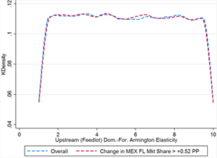
We first run the simulation using our calculated ad valorem equivalents for COOL compliance costs. We report the distribution of total changes in market shares, as well as the decomposition of effects by type, in tables 5 and 6. The means and ranges of the Armington and information effects are nearly identical for all countries at both levels, and the market expansion effects are very small for Canada and Mexico, on the order of 0.0001 percentage points. While the Armington and information effects have very similar overall distributions, they are only simultaneously of the same sign and general magnitude when the domestic-foreign Armington elasticity is near the middle of its possible range of values. As illustrated in figure 14, when the elasticity takes a value near either tail of the distribution, the two effects diverge. Although we only show the effect on Canada’s market share at the feedlot level here, we obtain similar results when comparing effects for all countries at all levels.

As seen in the data, in this round of simulations Canada and Mexico do not gain back their claimed losses in market share with the repeal of COOL even under extremely relaxed assumptions on initial market shares and Armington elasticities. The largest gain in market share for either Canada or Mexico is less than 0.12 percentage points at the upstream level and 0.23 percentage points at the downstream level. These upper bound estimates are significantly lower than what either Canada or Mexico claim in their WTO filings. On average, the effects are even smaller; Canada gains only 0.023 points at the upstream level and 0.011 at the downstream, and Mexico gains 0.056 and 0.114 percentage points at the upstream and downstream levels, respectively. Figures 5 and 6 illustrate the distribution of overall market share effects.

To determine the conditions under which the repeal of COOL would generate market share gains in line with Canada and Mexico’s claims, we run a second set of 100,000 simulations assuming that COOL compliance costs are an order of magnitude higher than in the first simulation[8]. Tables 7 and 8 report the decomposition of effects on market shares in this second round, and figures 7 and 8 illustrate the distributional results. In the downstream, the total market share changes were almost always greater than the “threshold” WTO values; in the upstream, however, the effects surpassed threshold values only for Mexico and only under certain assumptions on parameter values.

For Canada at the feedlot level the maximum market share increase is only 0.35 percentage points; there are still no cases where the gains reach or surpass the threshold value of 0.46 percentage points. Canada does, however, always gain back its stated level of damages in the downstream; in fact, the minimum overall gain in Canada’s downstream market share is nearly 0.07 percentage points higher than the threshold. In 61% of cases, Mexico reaches the threshold level at both the upstream and downstream levels, although it reaches the threshold in the downstream in over 95.7% of cases.

On average, Canada gains 0.250 percentage points in the upstream and 1.35 in the downstream, while Mexico gains 0.648 in the upstream and 1.614 in the downstream. These results suggest that raising the AVE tariff estimate by an order of magnitude is sufficient to generate downstream market share gains of corresponding magnitude to the WTO filings, when accounting for changes in both production costs and substitution elasticities. Notably, while on average the market share effects are much greater in the second simulation, the total ranges of effects are also much wider.

To illustrate the value of the Monte Carlo simulation in estimating policy effects, we discuss the distribution of Armington effects, which vary more across the WTO thresholds than the total market share changes. When considering only the Armington effects, increasing the magnitude of COOL compliance costs generates gains in line with the WTO filings only under certain conditions. For Canada, the Armington effect on changes in market share exceeds 0.46 percentage points in the upstream in only 45 cases (0.045%). In the downstream, however, the Armington effect meets or exceeds 0.31 percentage points in 68% of cases. Overall, the threshold values are met at both levels in only 0.03% of cases. For Mexico, the Armington effect by itself generates the necessary market share gains in 16% of cases in the upstream and 57% in the downstream, though with an overlap in only 9.5% of cases.

The following sections discuss the differences in the distribution of parameters between the overall set and the “threshold” set of cases, where the Armington effects are large enough to account for the damages filed with the WTO.  Unless stated otherwise, all differences in means are statistically significant.

Cases where Canada’s upstream Armington market share gains are greater than 0.46 percentage points

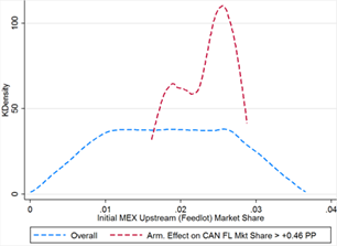
Canada recoups more than its claimed damages in upstream market share through Armington effects in only 45 cases. Strict assumptions must be placed on both market shares and Armington elasticities in order to generate sufficiently high gains (see table 9). Canada’s initial feedlot market share is always greater than 1.76%, at the top end of the overall distribution, and thus initial US upstream share is always less than 96.5%. Mexico’s share is bounded between 1.6% and 2.9%, near the center of its overall distribution (see figure 9C).

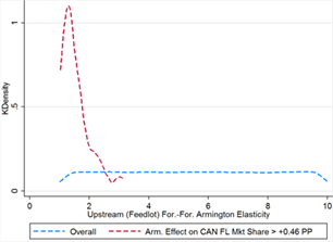
One must also assume that substitution between domestic and foreign cattle is almost perfectly elastic (alpha > 9.2) but that substitution between Canadian and Mexican cattle is relatively inelastic (beta < 3.2) in order to generate Canadian upstream market share gains greater than 0.46 percentage points in this model. Canada benefits from a low foreign-foreign Armington elasticity because its relative cost of COOL compliance is lower; Canadian cattle are more valuable than Mexican cattle on import and thus their fixed costs per head are more diluted when converting to an AVE tariff. When COOL is repealed, therefore, the relative price of Canadian cattle versus Mexican cattle increases (given that initial prices in the model are normalized to one) and Canadian market share suffers from high substitutability between foreign varieties.

Cases where Mexico’s upstream Armington market share gains are greater than 0.52 percentage points

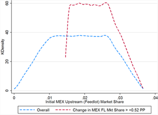
The positive Armington effect on Mexico’s feedlot market share gains is greater than 0.52 percentage points in 16% of cases. Both high initial market share and relatively high domestic-foreign and foreign-foreign Armington elasticities contribute to higher gains. According to the simulation results, in order to generate gains that surpass the threshold value one must assume that the domestic-foreign Armington elasticity is greater than 4.76 and that Mexico’s initial market share is greater than 1.5% (see table 10).

In addition to being bounded at the low end at 4.76, and the distribution of domestic-foreign Armington elasticities in the threshold cases is also heavily skewed to the right (see figure 10D). The average foreign-foreign Armington elasticity is only slightly higher in the threshold cases and till spans the full range of values, but the distribution is skewed right as well (figure 10E).

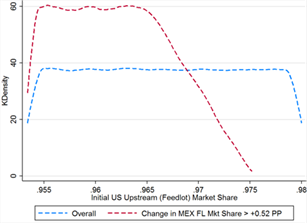
In the threshold cases Mexico’s initial feedlot market share is significantly higher and somewhat more normally distributed around a greater mean, 2.7% versus 1.8% overall (figure 10C). Consequently, initial US feedlot market share is never greater than 97.5% in the threshold cases, and Canada’s feedlot market share is also slightly lower on average.


Cases where Canada’s downstream Armington market share gains are greater than 0.31 percentage points

Canada’s downstream Armington market share gains surpass the threshold in over two-thirds of cases (68%). Because of this, none of the sampled parameters of interest, save for domestic-foreign Armington elasticity, are very different in distribution from the overall set of cases (see figures 11A-11E). In the threshold cases, the domestic-foreign Armington elasticity is bounded from below at 2.578 (see table 11), though it is still fairly uniformly distributed over its more limited range.

Cases where Mexico’s downstream Armington market share gains are greater than 0.49 percentage points

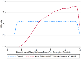
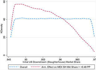
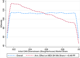
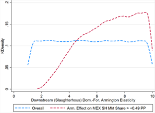
Mexico actually gains more than its claimed downstream market share losses through Armington effects alone in 57% of cases. Although this occurs at virtually all values of the primary parameters (domestic-foreign Armington elasticity is bounded from below at 1.694 and initial Mexican market share at 0.4%, see table 12), it is much more likely when Mexico’s initial market share is higher and when both domestic-foreign and foreign-foreign Armington elasticities are greater. Initial US downstream market share is heavily skewed left, with much lower density at the high end of the distribution (see figure 12A), and domestic-foreign Armington elasticity is similarly skewed right in addition to having slightly stricter bounds in the threshold cases (figure 12D).


The Information Effect

As previously stated, when accounting for all three kinds of market share effects, Canada and Mexico’s gains surpass the threshold in many more cases overall. Since the market expansion effects are still very small in the higher AVE round, the majority of this boost in gains comes from the inclusion of the information effect.

The exception to this boost is Canada’s change in upstream market share, which diminishes when accounting for changes in consumer information. Because the Armington elasticities must reach extreme values in order for Canada’s share to cross the threshold in the upstream, in the cases where the Armington effect is large enough the information effect on Canada’s upstream market share is always negative, bounded between -0.13 and -0.19 percentage points (see table 9). Thus, although when examining only Armington effects Canada does surpass the threshold in a very small subset of cases, it never does so when examining total effects.

When all three effects are accounted for, larger initial market share appears to be the single key factor in determining Mexico’s gains from COOL repeal. In the threshold cases, Mexico’s initial upstream market share is significantly higher in the threshold cases, 0.023 on average versus 0.018 overall (see table 13). The shape of the distribution is actually very similarly uniform between the overall and threshold set of cases (see figure 13C), but in the threshold cases Mexico’s initial market share is never less than 0.015 percentage points. Interestingly, when the information effect is also accounted for, the influence of the Armington elasticities disappears; as seen in figures 13D and 13E, the distributions of elasticities between the overall and threshold cases are nearly identical.

Conclusion

We introduce a vertically integrated, nested CES model to estimate the impacts of changes in COOL regulations. The vertical structure makes the standard CES model applicable for analyzing vertically integrated markets with both forward and backward linkages. We further incorporate a Monte Carlo simulation that allows the user to draw parameter values from a continuous uniform distribution. This allows for the introduction of uncertainty into parameter estimates and reduces the ex-ante research burden of economists by only requiring them to provide ranges for their parameter estimates. Moreover, it allows the user to produce a probability distribution of policy effects and determine how sensitive outcomes are to changes in parameter values. The latter is particularly important when outcome estimates cross important thresholds. In these cases, it is important to determine what factors drive these outcomes and what factors are irrelevant.

Furthermore, we are able to contribute to the literature by decomposing the effect of the repeal of COOL on market share through the change in relative prices (Armington effect), beef market expansion, and the change in information available to consumers. We show that the information effect is, on average, as large as the traditional Armington effect. Moreover, because these two effects dominate at different elasticity values, we show that by accounting for the information effect the estimates of the change in market share are robust to the choice of Armington elasticities. By contrast, initial market share does affect the magnitude of change in final market share from the repeal of COOL.

As an illustrative case, we apply the model to a recent change in COOL regulations. We show that the increased foreign market share following the repeal of COOL requirements only corresponds to the values claimed in WTO filings in cases where COOL compliance costs are an order of magnitude larger than USDA estimates. Moreover, we illustrate that the general magnitude of the results are robust to parameterization, and vary across foreign producers and sectors of the vertically integrated market. This result demonstrates the importance of correctly incorporating the vertical structure of a market and capturing all of the pathways through which a policy change can affect the outcome of interest.


Appendix A


We begin with a non-linear Armington model with n varieties. From Armington (1969) it can be shown that the demand for variety
i{ 1,n } MathType@MTEF@5@5@+= feaagKart1ev2aqatCvAUfeBSjuyZL2yd9gzLbvyNv2CaerbuLwBLn hiov2DGi1BTfMBaeXatLxBI9gBaerbd9wDYLwzYbItLDharqqtubsr 4rNCHbGeaGqiVCI8FfYJH8YrFfeuY=Hhbbf9v8qqaqFr0xc9pk0xbb a9q8WqFfeaY=biLkVcLq=JHqpepeea0=as0Fb9pgeaYRXxe9vr0=vr 0=vqpWqaaeaabiGaciaacaqabeaadaqaaqaaaOqaaabaaaaaaaaape GaamyAaiabgIGiopaacmaapaqaa8qacaaIXaGaaiilaiaad6gaaiaa wUhacaGL9baaaaa@3D2C@  is given by

x i = [ γ i P i ] σ P σ1 Y= γ i σ P i σ P σ1 Y MathType@MTEF@5@5@+= feaagKart1ev2aqatCvAUfeBSjuyZL2yd9gzLbvyNv2CaerbuLwBLn hiov2DGi1BTfMBaeXatLxBI9gBaerbd9wDYLwzYbItLDharqqtubsr 4rNCHbGeaGqiVCI8FfYJH8YrFfeuY=Hhbbf9v8qqaqFr0xc9pk0xbb a9q8WqFfeaY=biLkVcLq=JHqpepeea0=as0Fb9pgeaYRXxe9vr0=vr 0=vqpWqaaeaabiGaciaacaqabeaadaqaaqaaaOqaaabaaaaaaaaape GaamiEa8aadaWgaaWcbaWdbiaadMgaa8aabeaak8qacqGH9aqpdaWa daWdaeaapeWaaSaaa8aabaWdbiabeo7aN9aadaWgaaWcbaWdbiaadM gaa8aabeaaaOqaa8qacaWGqbWdamaaBaaaleaapeGaamyAaaWdaeqa aaaaaOWdbiaawUfacaGLDbaapaWaaWbaaSqabeaapeGaeq4WdmhaaO Gaamiua8aadaahaaWcbeqaa8qacqaHdpWCcqGHsislcaaIXaaaaOGa amywaiabg2da9iabeo7aN9aadaqhaaWcbaWdbiaadMgaa8aabaWdbi abeo8aZbaakiaadcfapaWaa0baaSqaa8qacaWGPbaapaqaa8qacqGH sislcqaHdpWCaaGccaWGqbWdamaaCaaaleqabaWdbiabeo8aZjabgk HiTiaaigdaaaGccaWGzbaaaa@58AD@      (A1)

where x i MathType@MTEF@5@5@+= feaagKart1ev2aqatCvAUfeBSjuyZL2yd9gzLbvyNv2CaerbuLwBLn hiov2DGi1BTfMBaeXatLxBI9gBaerbd9wDYLwzYbItLDharqqtubsr 4rNCHbGeaGqiVCI8FfYJH8YrFfeuY=Hhbbf9v8qqaqFr0xc9pk0xbb a9q8WqFfeaY=biLkVcLq=JHqpepeea0=as0Fb9pgeaYRXxe9vr0=vr 0=vqpWqaaeaabiGaciaacaqabeaadaqaaqaaaOqaaabaaaaaaaaape GaamiEa8aadaWgaaWcbaWdbiaadMgaa8aabeaaaaa@3851@  is quantity demanded of variety i, γ i MathType@MTEF@5@5@+= feaagKart1ev2aqatCvAUfeBSjuyZL2yd9gzLbvyNv2CaerbuLwBLn hiov2DGi1BTfMBaeXatLxBI9gBaerbd9wDYLwzYbItLDharqqtubsr 4rNCHbGeaGqiVCI8FfYJH8YrFfeuY=Hhbbf9v8qqaqFr0xc9pk0xbb a9q8WqFfeaY=biLkVcLq=JHqpepeea0=as0Fb9pgeaYRXxe9vr0=vr 0=vqpWqaaeaabiGaciaacaqabeaadaqaaqaaaOqaaabaaaaaaaaape Gaeq4SdC2damaaBaaaleaapeGaamyAaaWdaeqaaaaa@38FB@  is a shift parameter, P i MathType@MTEF@5@5@+= feaagKart1ev2aqatCvAUfeBSjuyZL2yd9gzLbvyNv2CaerbuLwBLn hiov2DGi1BTfMBaeXatLxBI9gBaerbd9wDYLwzYbItLDharqqtubsr 4rNCHbGeaGqiVCI8FfYJH8YrFfeuY=Hhbbf9v8qqaqFr0xc9pk0xbb a9q8WqFfeaY=biLkVcLq=JHqpepeea0=as0Fb9pgeaYRXxe9vr0=vr 0=vqpWqaaeaabiGaciaacaqabeaadaqaaqaaaOqaaabaaaaaaaaape Gaamiua8aadaWgaaWcbaWdbiaadMgaa8aabeaaaaa@3829@  is the price of variety i, P is the price index of the composite good, σ MathType@MTEF@5@5@+= feaagKart1ev2aqatCvAUfeBSjuyZL2yd9gzLbvyNv2CaerbuLwBLn hiov2DGi1BTfMBaeXatLxBI9gBaerbd9wDYLwzYbItLDharqqtubsr 4rNCHbGeaGqiVCI8FfYJH8YrFfeuY=Hhbbf9v8qqaqFr0xc9pk0xbb a9q8WqFfeaY=biLkVcLq=JHqpepeea0=as0Fb9pgeaYRXxe9vr0=vr 0=vqpWqaaeaabiGaciaacaqabeaadaqaaqaaaOqaaabaaaaaaaaape Gaeq4Wdmhaaa@37CF@  is the elasticity of substitution between varieties, and Y is total expenditure in the market.

The market share of variety i in the market for the composite good is given by

φ i = x i P i j=1 n x j P j MathType@MTEF@5@5@+= feaagKart1ev2aqatCvAUfeBSjuyZL2yd9gzLbvyNv2CaerbuLwBLn hiov2DGi1BTfMBaeXatLxBI9gBaerbd9wDYLwzYbItLDharqqtubsr 4rNCHbGeaGqiVCI8FfYJH8YrFfeuY=Hhbbf9v8qqaqFr0xc9pk0xbb a9q8WqFfeaY=biLkVcLq=JHqpepeea0=as0Fb9pgeaYRXxe9vr0=vr 0=vqpWqaaeaabiGaciaacaqabeaadaqaaqaaaOqaaabaaaaaaaaape GaeqOXdO2damaaBaaaleaapeGaamyAaaWdaeqaaOWdbiabg2da9maa laaapaqaa8qacaWG4bWdamaaBaaaleaapeGaamyAaaWdaeqaaOWdbi aadcfapaWaaSbaaSqaa8qacaWGPbaapaqabaaakeaapeWaaubmaeqa l8aabaWdbiaadQgacqGH9aqpcaaIXaaapaqaa8qacaWGUbaan8aaba WdbiabggHiLdaakiaadIhapaWaaSbaaSqaa8qacaWGQbaapaqabaGc peGaamiua8aadaWgaaWcbaWdbiaadQgaa8aabeaaaaaaaa@4987@      (A2)

where x i P i MathType@MTEF@5@5@+= feaagKart1ev2aqatCvAUfeBSjuyZL2yd9gzLbvyNv2CaerbuLwBLn hiov2DGi1BTfMBaeXatLxBI9gBaerbd9wDYLwzYbItLDharqqtubsr 4rNCHbGeaGqiVCI8FfYJH8YrFfeuY=Hhbbf9v8qqaqFr0xc9pk0xbb a9q8WqFfeaY=biLkVcLq=JHqpepeea0=as0Fb9pgeaYRXxe9vr0=vr 0=vqpWqaaeaabiGaciaacaqabeaadaqaaqaaaOqaaabaaaaaaaaape GaamiEa8aadaWgaaWcbaWdbiaadMgaa8aabeaak8qacaWGqbWdamaa BaaaleaapeGaamyAaaWdaeqaaaaa@3A88@  is the total expenditure on variety i.

To find x i P i MathType@MTEF@5@5@+= feaagKart1ev2aqatCvAUfeBSjuyZL2yd9gzLbvyNv2CaerbuLwBLn hiov2DGi1BTfMBaeXatLxBI9gBaerbd9wDYLwzYbItLDharqqtubsr 4rNCHbGeaGqiVCI8FfYJH8YrFfeuY=Hhbbf9v8qqaqFr0xc9pk0xbb a9q8WqFfeaY=biLkVcLq=JHqpepeea0=as0Fb9pgeaYRXxe9vr0=vr 0=vqpWqaaeaabiGaciaacaqabeaadaqaaqaaaOqaaabaaaaaaaaape GaamiEa8aadaWgaaWcbaWdbiaadMgaa8aabeaak8qacaWGqbWdamaa BaaaleaapeGaamyAaaWdaeqaaaaa@3A88@  we multiply quantity demanded (A1) by the price of i:

x i P i = γ i σ P i 1σ P σ1 Y MathType@MTEF@5@5@+= feaagKart1ev2aqatCvAUfeBSjuyZL2yd9gzLbvyNv2CaerbuLwBLn hiov2DGi1BTfMBaeXatLxBI9gBaerbd9wDYLwzYbItLDharqqtubsr 4rNCHbGeaGqiVCI8FfYJH8YrFfeuY=Hhbbf9v8qqaqFr0xc9pk0xbb a9q8WqFfeaY=biLkVcLq=JHqpepeea0=as0Fb9pgeaYRXxe9vr0=vr 0=vqpWqaaeaabiGaciaacaqabeaadaqaaqaaaOqaaabaaaaaaaaape GaamiEa8aadaWgaaWcbaWdbiaadMgaa8aabeaak8qacaWGqbWdamaa BaaaleaapeGaamyAaaWdaeqaaOWdbiabg2da9iabeo7aN9aadaqhaa WcbaWdbiaadMgaa8aabaWdbiabeo8aZbaakiaadcfapaWaa0baaSqa a8qacaWGPbaapaqaa8qacaaIXaGaeyOeI0Iaeq4WdmhaaOGaamiua8 aadaahaaWcbeqaa8qacqaHdpWCcqGHsislcaaIXaaaaOGaamywaaaa @4B8C@      (A3)

Substituting (A3) into the market share equation (A2), we obtain

φ i = γ i σ P i 1σ × P σ1 Y P σ1 Y× j=1 n γ j σ P j 1σ = γ i σ P i 1σ j=1 n γ j σ P j 1σ MathType@MTEF@5@5@+= feaagKart1ev2aqatCvAUfeBSjuyZL2yd9gzLbvyNv2CaerbuLwBLn hiov2DGi1BTfMBaeXatLxBI9gBaerbd9wDYLwzYbItLDharqqtubsr 4rNCHbGeaGqiVCI8FfYJH8YrFfeuY=Hhbbf9v8qqaqFr0xc9pk0xbb a9q8WqFfeaY=biLkVcLq=JHqpepeea0=as0Fb9pgeaYRXxe9vr0=vr 0=vqpWqaaeaabiGaciaacaqabeaadaqaaqaaaOqaaabaaaaaaaaape GaeqOXdO2damaaBaaaleaapeGaamyAaaWdaeqaaOWdbiabg2da9maa laaapaqaa8qacqaHZoWzpaWaa0baaSqaa8qacaWGPbaapaqaa8qacq aHdpWCaaGccaWGqbWdamaaDaaaleaapeGaamyAaaWdaeaapeGaaGym aiabgkHiTiabeo8aZbaakiabgEna0kaadcfapaWaaWbaaSqabeaape Gaeq4WdmNaeyOeI0IaaGymaaaakiaadMfaa8aabaWdbiaadcfapaWa aWbaaSqabeaapeGaeq4WdmNaeyOeI0IaaGymaaaakiaadMfacqGHxd aTdaqfWaqabSWdaeaapeGaamOAaiabg2da9iaaigdaa8aabaWdbiaa d6gaa0WdaeaapeGaeyyeIuoaaOGaeq4SdC2damaaDaaaleaapeGaam OAaaWdaeaapeGaeq4WdmhaaOGaamiua8aadaqhaaWcbaWdbiaadQga a8aabaWdbiaaigdacqGHsislcqaHdpWCaaaaaOGaeyypa0ZaaSaaa8 aabaWdbiabeo7aN9aadaqhaaWcbaWdbiaadMgaa8aabaWdbiabeo8a ZbaakiaadcfapaWaa0baaSqaa8qacaWGPbaapaqaa8qacaaIXaGaey OeI0Iaeq4WdmhaaaGcpaqaa8qadaqfWaqabSWdaeaapeGaamOAaiab g2da9iaaigdaa8aabaWdbiaad6gaa0WdaeaapeGaeyyeIuoaaOGaeq 4SdC2damaaDaaaleaapeGaamOAaaWdaeaapeGaeq4WdmhaaOGaamiu a8aadaqhaaWcbaWdbiaadQgaa8aabaWdbiaaigdacqGHsislcqaHdp WCaaaaaaaa@80C9@     (A4)

This result holds regardless of any assumptions on the price elasticity of supply.


Fig 5. Distributions of Key Parameters for Cases where Decline in U.S. Market Share Exceeds 1 Pct Pt

 
Figures


Figure 1: One-sector, CES model diagram
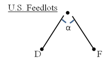
Title: Figure 1 - Description: A single node representing U.S. feedlots faces two choice branches: they will purchase either domestic or foreign cattle. The acute angle between the branches, labeled alpha, represents the elasticity of substitution between domestic and foreign cattle.

Figure 2: One-sector, nested CES model diagram

Title: Figure 2 - Description: A single node representing U.S. feedlots faces two choice branches: they will purchase either domestic or foreign cattle. Within the foreign branch is nested a second choice node: the feedlot owner will purchase either Mexican or Canadian cattle. The elasticity of substitution between domestic and foreign cattle is alpha, while the elasticity of substitution between Mexican and Canadian cattle is beta.

Figure 3: Two sector, vertically integrated, nested CES model diagram
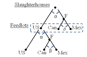
Title: Figure 3 - Description: A single node representing U.S. slaughterhouses faces the choice of purchasing cattle from either domestic or foreign feedlots, with elasticity of substitution sigma. Nested within the foreign feedlot branch is the choice between cattle from Canadian or Mexican feedlots, with elasticity of substitution theta. The U.S. feedlot branch is connected to the nested choice structure from figure 2, where cattle in U.S. feedlots can come from domestic or foreign sources.

Figure 4: Cattle Market Path

Title: Figure 4 - Description: U.S. feedlots contain U.S.-born cattle and also receive cattle from Canada and Mexico. All three types of cattle, once they are large enough, “flow” down to U.S. slaughterhouses, where they are supplemented by fed cattle from Canadian feedlots and other U.S. sources.


Figure 5: Total Effects on the Upstream Sector for a Low AVE


Title: Figure 5 - Description: Change in U.S. upstream market share in the low tariff simulation is distributed in a symmetrical bell shape around a peak of -0.06 percentage points, with a range between -0.13 and 0 percentage points.
Change in Canadian upstream market share is distributed somewhat uniformly between 0.015 percentage points and 0.033 percentage points.
Change in Mexican upstream market share is distributed somewhat uniformly in the center of its distribution, with symmetrical downward-sloping probability density at the low and high ends; the center is near 0.06 percentage points and the range is between 0 and 0.12 percentage points.
When all three kernel density plots are displayed in the same graph, the Canadian distribution is concentrated very tightly at the low end of the Mexican distribution, which is much flatter. The U.S. distribution is similar in shape and range to the Mexican distribution; the two distributions look like reflections of each other across the 0 percentage point mark.


Figure 6: Total Effects on the Downstream Sector for a Low AVE


Title: Figure 6 - Description: Change in U.S. downstream market share in the low tariff simulation is symmetrically distributed in a bell shape around a mean of -0.2 percentage points, with a range from -0.32 to -0.11 percentage points.
Change in Canadian downstream market share is symmetrically distributed in a skinny bell shape around a mean of 0.11 percentage points, with a range between 0.05 and 0.18 percentage points.
The density plot of changes in Mexican downstream market share is again somewhat flat in the middle, though slightly tilted up towards the higher end, and slopes sharply downward near its extrema. The mean is at +0.11 percentage points and the range is between 0 and 0.23 percentage points.
When all three kernel density plots are displayed in the same graph, the Canadian distribution is nested right in the center of the Mexican distribution. The U.S. distribution again looks similar to the Mexican distribution, though it is taller and rounder on top and situated in the far negative side of the value axis.


Figure 7: Total Effects on the Upstream Sector for a High AVE


Title: Figure 7 - Description: Change in U.S. upstream market share in the high tariff simulation is distributed in a symmetrical bell shape around a peak of -0.65 percentage points, with a range between -1.4 and 0.05 percentage points.
Change in Canadian upstream market share is distributed somewhat uniformly between 0.15 percentage points and 0.35 percentage points.
Change in Mexican upstream market share is distributed somewhat uniformly in the center of its distribution, with symmetrical downward-sloping probability density at the low and high ends; the center is near 0.65 percentage points and the range is between 0 and 1.29 percentage points.
When all three kernel density plots are displayed in the same graph, the Canadian distribution is concentrated very tightly at the low end of the Mexican distribution, which is much flatter. The U.S. distribution is very similar in shape and range to the Mexican distribution; the two distributions look like reflections of each other across the 0 percentage point mark.


Figure 8: Total Effects on the Downstream Sector for a High AVE
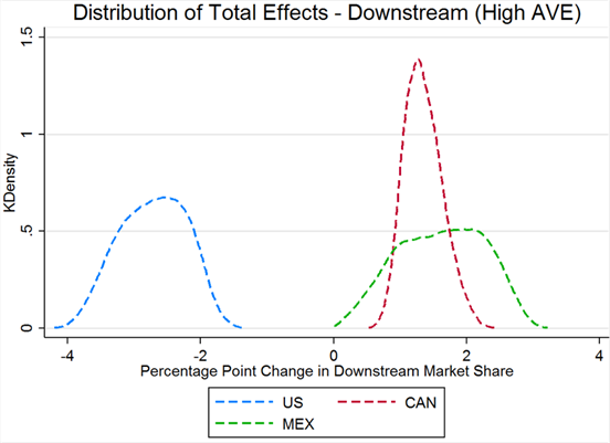


Title: Figure 8 - Description: Change in U.S. downstream market share in the high tariff simulation is symmetrically distributed in a flattened bell shape around a mean of -2.72 percentage points, with a range from -4.19 to -1.36 percentage points.
Change in Canadian downstream market share is distributed in a pointed bell shape with a long right tail around a mode of 1.3 percentage points, with a range between 0.53 and 2.45 percentage points.
The density plot of changes in Mexican downstream market share is again somewhat flat in the middle, though slightly tilted up towards the higher end, and slopes sharply downward near its extrema. The mean is at 1.61 percentage points and the range is between 0 and 3.22 percentage points.
When all three kernel density plots are displayed in the same graph, the Canadian distribution is nested right in the center of the Mexican distribution. The U.S. distribution again looks similar to the Mexican distribution, though it is taller and rounder on top and situated in the far negative side of the value axis.


Comparative Kernel Density Plots


Figure 9A                                                                   Figure 9B
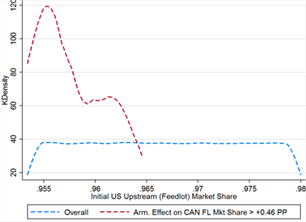
Title: Figure 9A - Description: Initial U.S. upstream market share is uniformly distributed between 95.3 and 98 percent in the high tariff simulation. In the subset of cases where the Armington effect on Canada’s upstream market share is greater than 0.46 percentage points, initial U.S. market share has a jagged density plot with one large and one small peak. This distribution is at the low end of its overall range, bounded from above at only 96.5 percent. The mode in these cases is near 95.5 percent.Title: Figure 9B - Description: Initial Canadian upstream market share is uniformly distributed between 1 and 2 percent in the high tariff simulation. In the subset of cases where the Armington effect on Canada’s upstream market share is greater than 0.46 percentage points, initial Canadian upstream market share has a jagged density plot with one large and one very small peak. This distribution is at the very high end of its overall range, bounded from below at 1.75 percent. The mode in these cases is near 2 percent.


Figure 9C                                                                   Figure 9D

Title: Figure 9C - Description: Initial Mexican upstream market share in the high tariff simulation has a density plot that is flat in the middle and linearly sloped on either side, ranging from 0 to 3.7 percent. In the subset of cases where the Armington effect on Canada’s upstream market share is greater than 0.46 percentage points, initial Mexican upstream market share has a density plot with one large and one small peak. This distribution is located near the center of its overall distribution, bounded from below at 1.6 percent and from above at 2.9 percent. The mode of this distribution is near 2.6 percent.Title: Figure 9D - Description: Upstream domestic-foreign Armington elasticity is uniformly distributed between 1 and 10 in the high tariff simulation. In the subset of cases where the Armington effect on upstream market share is greater than 0.46 percentage points, the density plot of the domestic-foreign Armington elasticity is bounded from below at 9.2 and has a mode very close to 10 where most of the observations are located.


Figure 9E

Title: Figure 9E - Description: Upstream foreign-foreign Armington elasticity is uniformly distributed between 1 and 10 in the high tariff simulation. In the subset of cases where the Armington effect on Canada’s upstream market share is greater than 0.46 percentage points, the density plot of the foreign-foreign Armington elasticity is bounded from above at 3.2 and has a single peak at its mode, near 1.9.


Figure 10A                                                                 Figure 10B

Title: Figure 10A - Description: Initial U.S. upstream market share is uniformly distributed between 95.3 and 98 percent in the high tariff simulation. In the subset of cases where the Armington effect on Mexico’s upstream market share is greater than 0.52 percentage points, the density plot of initial U.S. market share peaks at 95.5 percent and gradually slopes down to an upper bound of 97.4 percent.Title: Figure 10B - Description: Initial Canadian upstream market share is uniformly distributed between 1 and 2 percent in the high tariff simulation. In the subset of cases where the Armington effect on Mexico’s upstream market share is greater than 0.52 percentage points, the density plot of initial upstream market share is heavily skewed towards the low end of the overall distribution, sloping downward rather than being flat.


Figure 10C                                                                 Figure 10D

Title: Figure 10C - Description: Initial Mexican upstream market share in the high tariff simulation has a probability distribution that is flat in the middle and linearly sloped on either side, ranging from 0 to 3.7 percent. In the subset of cases where the Armington effect on Mexico’s upstream market share is greater than 0.52 percentage points, initial Mexican feedlot market share has a roughly triangular symmetrical density plot bounded from below at 1.5 percent and centered near 2.8 percent.Title: Figure 10D - Description: Upstream domestic-foreign Armington elasticity is uniformly distributed between 1 and 10 in the high tariff simulation. In the subset of cases where the Armington effect on upstream market share is greater than 0.52 percentage points, the density plot of the domestic-foreign Armington elasticity is bounded from below at 4.7 and gradually slopes upward to a peak near 9.7.


Figure 10E

Title: Figure 10E - Description: Upstream foreign-foreign Armington elasticity is uniformly distributed between 1 and 10 in the high tariff simulation. In the subset of cases where the Armington effect on upstream market share is greater than 0.52 percentage points, the density plot of the foreign-foreign Armington elasticity is heavily skewed towards the high end of the overall distribution, sloping upwards rather than being flat.


Figure 11A                                                                 Figure 11B

Title: Figure 11A - Description: Initial U.S. downstream market share is uniformly distributed between 94.6 percent and 97 percent in the high tariff simulation. In the subset of cases where the Armington effect on Canadian downstream market share is greater than 0.31 percentage points, the density plot of initial U.S. market share is slightly skewed to the high end of the overall distribution, gently sloping upward rather than being flat.Title: Figure 11B - Description: Initial Canadian downstream market share is uniformly distributed between 2.1 and 3 percent in the high tariff simulation. In the subset of cases where the Armington effect on Canadian downstream market share is greater than 0.31 percentage points, the density plot of initial Canadian market share is slightly skewed to the high end of the overall distribution, gently sloping upward rather than being flat.


Figure 11C                                                                 Figure 11D

Title: Figure 11C - Description: Initial Mexican downstream market share in the high tariff simulation has a distribution that is flat in the middle and linearly sloped on either side, bounded between 0 to 3.3 percent. In the subset of cases where the Armington effect on Canadian downstream market share is greater than 0.31 percentage points, the density plot of initial Mexican market shares is practically identical to that of the overall set of cases, albeit very slightly skewed to the low end of the overall distribution.Title: Figure 11D - Description: Downstream domestic-foreign Armington elasticity is uniformly distributed between 1 and 10 in the high tariff simulation. In the subset of cases where the Armington effect on Canadian downstream market share is greater than 0.31 percentage points, the density plot of domestic-foreign Armington elasticity is bounded from below at 2.5. It slopes sharply upward between 2.5 and 5, and is uniform between 5 and 10.


Figure 11E

Title: Figure 11E - Description: Downstream foreign-foreign Armington elasticity is uniformly distributed between 1 and 10 in the high tariff simulation. In the subset of cases where the Armington effect on Canadian downstream market share is greater than 0.31 percentage points, the density plot of foreign-foreign Armington elasticity is slightly skewed to the low end of the overall distribution, sloping downward instead of being flat.


Figure 12A                                                                 Figure 12B

Title: Figure 12A - Description: Initial U.S. downstream market share is uniformly distributed between 94.6 percent and 97 percent in the high tariff simulation. In the subset of cases where the Armington effect on Mexico’s downstream market share is greater than 0.49 percentage points, the density plot of initial U.S. market share peaks at the very low end of the overall distribution and then slopes downward in a concave fashion, approaching zero density at 97 percent.Title: Figure 12B - Description: Initial Canadian downstream market share is uniformly distributed between 2.1 and 3 percent in the high tariff simulation. In the subset of cases where the Armington effect on Mexico’s downstream market share is greater than 0.49 percentage points, the density plot of initial Canadian market share is skewed to the low end of the overall distribution, sloping downward rather than being flat.


Figure 12C                                                                 Figure 12D

Title: Figure 12C - Description: Initial Mexican downstream market share in the high tariff simulation has a distribution that is flat in the middle and linearly sloped on either side, bounded between 0 to 3.3 percent. In the subset of cases where the Armington effect on Mexico’s downstream market share is greater than 0.49 percentage points, the density plot of initial Mexican market shares is bounded from below at 0.4 percent, sloping upward in a rough bell shape to a mode of 2.4 percent and then decreasing linearly to the upper bound of 3.3 percent.Title: Figure 12D - Description: Downstream domestic-foreign Armington elasticity is uniformly distributed between 1 and 10 in the high tariff simulation. In the subset of cases where the Armington effect on Mexico’s downstream market share is greater than 0.49 percentage points, the density plot of domestic-foreign Armington elasticity is bounded from below at 1.7. It slopes upward in an S-shape to a mode at the very high end of the overall distribution.


Figure 12E

Title: Figure 12E - Description: Downstream foreign-foreign Armington elasticity is uniformly distributed between 1 and 10 in the high tariff simulation. In the subset of cases where the Armington effect on Mexico’s downstream market share is greater than 0.49 percentage points, the density plot of foreign-foreign Armington elasticity is slightly skewed to the high end of the overall distribution, sloping upward instead of being flat.


Figure 13A                                                                 Figure 13B

Title: Figure 13A - Description: Initial U.S. upstream market share is uniformly distributed between 95.3 percent and 98 percent in the high tariff simulation. In the subset of cases where the total change in Mexico’s upstream market share is greater than 0.52 percentage points, initial U.S. market share has uniform distribution between 95 percent and 96.5 percent which then slopes linearly downward to an upper bound of 97.5 percent.Title: Figure 13B - Description: Initial Canadian upstream market share is uniformly distributed between 1 and 2 percent in the high tariff simulation. In the subset of cases where the total change in Mexico’s upstream market share is greater than 0.52 percentage points, the density plot of Canada’s initial market share is skewed to the low end of the overall distribution, sloping downward rather than being flat.


Figure 13C                                                                 Figure 13D

Title: Figure 13C - Description: Initial Mexican upstream market share in the high tariff simulation has a distribution that is flat in the middle and linearly sloped on either side, bounded between 0 to 3.5 percent. In the subset of cases where the total change in Mexico’s upstream market share is greater than 0.52 percentage points, initial Mexican market share is identically distributed to the overall case but truncated from below at 1.5 percent.Title: Figure 13D - Description: Upstream domestic-foreign Armington elasticity is uniformly distributed between 1 and 10 in the high tariff simulation. There is no difference in distribution between the overall set of cases and the set of cases where the total change in Mexico’s upstream market share is greater than 0.52 percentage points.


Figure 13E

Title: Figure 13E - Description: Upstream foreign-foreign Armington elasticity is uniformly distributed between 1 and 10 in the high tariff simulation. There is no difference in distribution between the overall set of cases and the set of cases where the total change in Mexico’s upstream market share is greater than 0.52 percentage points.


Figure 14

Title: Figure 14 - Description: The magnitudes of both the Armington and information effects on Canada’s upstream market share are symmetrically distributed in bell shapes. The two distributions overlap more the closer the domestic-foreign Armington elasticity is to its mean value of 5.5, and diverge as the elasticity becomes more extreme. When the domestic-foreign Armington elasticity is less than three, the density plot of Armington effects is completely to the left of the density plot of information effects, and is more tightly distributed around its mean. When the domestic-foreign Armington elasticity is between 3 and 5, there is overlap between the two density plots between 0 and 0.2 percentage points on the value axis.
When the domestic-foreign Armington elasticity is between 5 and 7, the two density plots are mostly overlapping, with the Armington effect distribution now slightly to the right of the information effect distribution.
When the domestic-foreign Armington elasticity is greater than seven, the density plot of information effects is now almost entirely to the left of the density plot of Armington effects and more tightly bounded, with minor overlap between the distributions between 0.13 and 0.18 percentage points.


Fig 5. Distributions of Key Parameters for Cases where Decline in U.S. Market Share Exceeds 1 Pct Pt

 
Tables


Table 1: Price per head (USD)

Price per head (USD)

USA

Canada

Mexico

Feeder Cattle

1,571.86

1,268.60

661.71

Feeder Cattle (value at slaughter)

2,161.25*

1,744.28

909.83

Fed Cattle

2,161.25

1,767.14

-

*U.S. feedlot “value added” ratio = 1.375


Table 2: Market Shares

Total value (in millions USD)

USA

Canada

Mexico

Feeder Cattle

40,067

621

737

Market Share at Feedlot

96.72%

1.50%

1.78%

Feeder Cattle (value at slaughter)

55,090

854

1,013

Fed Cattle (additional)

3,458

713

-

Total (at slaughterhouse)

58,548

1,567

1,013

Market Share at Slaughterhouse

95.78%

2.56%

1.66%


Table 3: Ad Valorem Tax Equivalents

Canadian Cost

Canadian Value

Canadian Tax

Mexican Cost

Mexican Value

Mexican Tax

$2.25

$1,268.60

0.177%

$2.25

$661.71

0.340%

$6.75*

$1,744.28

0.454%

$6.75

$909.83

0.742%

$9.00**

$1,767.14

0.454%

$6.75

$909.83

0.742%


* 54.8% of Canadian cattle in U.S. slaughterhouses come from U.S. feedlots.

** 45.2% of Canadian cattle in U.S. slaughterhouses come from Canadian feedlots.


Table 4: Bounds of Parameter (Estimates Both Experiments)

Variable

Lower Bound

Upper Bound

Domestic-Foreign Elasticity of Substitution (Alpha)

1

10

Foreign-Foreign Elasticity of Substitution (Beta)

1

10

Domestic-Foreign Elasticity of Substitution (Sigma)

1

10

Foreign-Foreign Elasticity of Substitution (Theta)

1

10

Beef-Not Beef Elasticity

1

6

Mkt Share US Feedlot (US)

0.953

0.980

Mkt Share US Feedlot (Canada)

0.010

0.020

Mkt Share US Feedlot (Mexico)

0.000

0.037

Mkt Share US Slaughterhouses (US)

0.946

0.970

Mkt Share US Slaughterhouses (Canada)

0.021

0.030

Mkt Share US Slaughterhouses (Mexico)

0.000

0.033

Beef Share in US Meat Mkt

0.48

0.48


Note: All drawn from continuous uniform distribution


Table 5: Feedlot Level Market Share Change Decomposition (Low AVE)

Country

Total
Change

Armington
Effect

Market
Expansion Effect

Information
Effect

USA

-0.057*

-0.039

0.021

-0.039


[-0.123,0.002]

[-0.123,-0.00005]

[0.0001,0.060]

[-0.122,-0.00001]

CAN

0.023

0.011

0.0003

0.011


[0.015,0.032]

[-0.015,0.045]

[0.000,0.001]

[-0.016,0.045]

MEX

0.056

0.028

0.0004

0.028


[0.0001,0.110]

[0.0001,0.105]

[0.000,0.002]

[0.00001,0.104]


* Changes are in percentage points. Minimum and maximum changes are in square brackets.


Table 6: Slaughterhouse Level Market Share Change Decomposition (Low AVE)

Country

Total
Change

Armington
Effect

Market Expansion Effect

Information
Effect

USA

-0.202*

-0.111

0.021

-0.112


[-0.312,-0.105]

[-0.308,-0.0002]

[0.0001,0.060]

[-0.310,-0.00001]

CAN

0.110

0.054

0.001

0.055


[-0.052,0.178]

[-0.034,0.174]

[0.000,0.002]

[-0.035,0.172]

MEX

0.114

0.056

0.0004

0.057


[0.0003,0.227]

[0.0001,0.213]

[0.000,0.002]

[0.0001,0.210]


* Changes are in percentage points. Minimum and maximum changes are in square brackets.


Table 7: Feedlot Level Market Share Change Decomposition (High AVE)

Country

Total
Change

Armington Effect

Market Expansion Effect

Information Effect

USA

-0.649*

-0.424

0.239

-0.465


[-1.405,0.049]

[-1.399,-0.0004]

[0.0007,0.733]

[-1.393,-0.0004]

CAN

0.250

0.122

0.004

0.124


[0.158,0.349]

[-0.159,0.505]

[0.00001,0.016]

[-0.197,0.478]

MEX

0.648

0.302

0.006

0.341


[0.002,1.289]

[0.0002,1.214]

[0.000,0.033]

[0.0008,1.212]


*
Changes are in percentage points. Minimum and maximum changes are in square brackets.


Table 8: Slaughterhouse Level Market Share Change Decomposition (High AVE)

Country

Total
Change

Armington Effect

Market Expansion Effect

Information Effect

USA

-2.715*

-1.342

0.235

-1.607


[-4.196,-1.355]

[-4.154,-0.002]

[0.001,0.700]

[-4.158,0.009]

CAN

1.350

0.642

0.008

0.700


[0.534,2.444]

[-0.343,2.291]

[0.0002,0.035]

[-0.587,2.370]

MEX

1.614

0.700

0.006

0.907


[0.008,3.219]

[0.001,2.859]

[0.000,0.046]

[0.003,2.955]


*
Changes are in percentage points. Minimum and maximum changes are in square brackets.


Table 9: Distribution of Variables When Armington Effect on Canada's Feedlot Market Share > +0.46 Percentage Points

Variable

Mean

Std. Dev.

Min

Max

Initial Feedlot Market Share

USA

0.958

0.003

0.953

0.965

Initial Feedlot Market Share

CAN

0.019

0.001

0.018

0.020

Initial Feedlot Market Share

MEX

0.023

0.004

0.016

0.029

Change in Feedlot Market Share (Pct Pt)

USA

-0.837

0.178

-1.214

-0.447

Change in Feedlot Market Share (Pct Pt)

CAN

0.318

0.011

0.289

0.335

Change in Feedlot Market Share (Pct Pt)

MEX

0.815

0.125

0.571

1.013

Market Expansion Effect on Feedlot Market Share (Pct Pt)

USA

0.280

0.154

0.009

0.631

Market Expansion Effect on Feedlot Market Share (Pct Pt)

CAN

0.007

0.004

0.0002

0.016

Market Expansion Effect on Feedlot Market Share (Pct Pt)

MEX

0.009

0.005

0.0003

0.023

Information Effect on Feedlot Market Share (Pct Pt)

USA

-0.042

0.027

-0.117

-0.011

Information Effect on Feedlot Market Share (Pct Pt)

CAN

-0.165

0.016

-0.197

-0.139

Information Effect on Feedlot Market Share (Pct Pt)

MEX

0.207

0.026

0.151

0.269

Armington Effect on Feedlot Market Share (Pct Pt)

USA

-1.074

0.116

-1.244

-0.858

Armington Effect on Feedlot Market Share (Pct Pt)

MEX

0.599

0.111

0.395

0.775

Upstream Domestic-Foreign Armington Elasticity


9.787

0.196

9.284

9.997

Upstream Foreign-Foreign Armington Elasticity


1.547

0.493

1.031

3.128

Note: 45 observations.


Table 10: Distribution of Variables When Armington Effect on Mexico's Feedlot Market Share > +0.52 Percentage Points


Variable

Mean

Std. Dev.

Min

Max

Initial Feedlot Market Share

USA

0.959

0.004

0.953

0.974

Initial Feedlot Market Share

CAN

0.014

0.003

0.010

0.020

Initial Feedlot Market Share

MEX

0.027

0.004

0.015

0.037

Change in Feedlot Market Share
(Pct Pt)

USA

-0.888

0.202

-1.401

-0.164

Change in Feedlot Market Share
(Pct Pt)

CAN

0.229

0.045

0.158

0.337

Change in Feedlot Market Share
(Pct Pt)

MEX

0.942

0.148

0.538

1.289

Market Expansion Effect on Feedlot Market Share (Pct Pt)

USA

0.269

0.160

0.001

0.730

Market Expansion Effect on Feedlot Market Share (Pct Pt)

CAN

0.005

0.003

0.0000

0.016

Market Expansion Effect on Feedlot Market Share (Pct Pt)

MEX

0.010

0.006

0.0000

0.033

Information Effect on Feedlot Market Share (Pct Pt)

USA

-0.249

0.174

-0.846

-0.001

Information Effect on Feedlot Market Share (Pct Pt)

CAN

0.004

0.072

-0.197

0.235

Information Effect on Feedlot Market Share (Pct Pt)

MEX

0.245

0.132

0.001

0.720

Armington Effect on Feedlot Market Share (Pct Pt)

USA

-0.909

0.159

-1.399

-0.535

Armington Effect on Feedlot Market Share (Pct Pt)

CAN

0.221

0.085

-0.003

0.505

Upstream Domestic-Foreign Armington Elasticity


8.303

1.152

4.763

10.000

Upstream Foreign-Foreign Armington Elasticity


6.089

2.531

1.013

10.000

Note: 16,066 observations.


Table 11: Distribution of Variables When Armington Effect on Canada's Slaughterhouse Market Share > +0.31 Percentage Points


Variable

Country

Mean

Std. Dev.

Min.

Max.

Initial Slaughterhouse Market Share

USA

0.958

0.007

0.946

0.970

Initial Slaughterhouse Market Share

CAN

0.026

0.003

0.021

0.030

Initial Slaughterhouse Market Share

MEX

0.016

0.007

0.000

0.033

Change in Slaughterhouse Market Share (Pct Pt)

USA

-2.697

0.506

-4.185

-1.355

Change in Slaughterhouse Market Share (Pct Pt)

CAN

1.374

0.289

0.553

2.444

Change in Slaughterhouse Market Share (Pct Pt)

MEX

1.580

0.654

0.008

3.219

Market Expansion Effect on Slaughterhouse Market Share (Pct Pt)

USA

0.241

0.147

0.001

0.700

Market Expansion Effect on Slaughterhouse Market Share (Pct Pt)

CAN

0.009

0.006

0.0000

0.035

Market Expansion Effect on Slaughterhouse Market Share (Pct Pt)

MEX

0.007

0.006

0.0000

0.046

Information Effect on Slaughterhouse Market Share (Pct Pt)

USA

-1.162

0.673

-3.472

0.009

Information Effect on Slaughterhouse Market Share (Pct Pt)

CAN

0.455

0.422

-0.587

2.035

Information Effect on Slaughterhouse Market Share (Pct Pt)

MEX

0.707

0.416

0.003

2.577

Armington Effect on Slaughterhouse Market Share (Pct Pt)

USA

-1.776

0.729

-4.154

-0.324

Armington Effect on Slaughterhouse Market Share (Pct Pt)

CAN

0.865

0.501

0.004

2.859

Armington Effect on Slaughterhouse Market Share (Pct Pt)

MEX

-1.776

0.729

-4.154

-0.324

Downstream Domestic-Foreign Armington Elasticity


6.890

1.844

2.578

10.000

Downstream Foreign-Foreign Armington Elasticity


5.252

2.587

1.010

10.000

Note: 68,032 observations.


Table 12: Distribution of Variables When Armington Effect on Mexico's Slaughterhouse Market Share > +0.49 Percentage Points


Variable

Country

Mean

Std. Dev.

Min.

Max.

Initial Slaughterhouse Market Share

USA

0.955

0.006

0.946

0.970

Initial Slaughterhouse Market Share

CAN

0.025

0.003

0.021

0.030

Initial Slaughterhouse Market Share

MEX

0.019

0.006

0.004

0.033

Change in Slaughterhouse Market Share (Pct Pt)

USA

-2.875

0.463

-4.185

-1.400

Change in Slaughterhouse Market Share (Pct Pt)

CAN

1.275

0.244

0.553

2.154

Change in Slaughterhouse Market Share (Pct Pt)

MEX

1.869

0.527

0.532

3.219

Market Expansion Effect on Slaughterhouse Market Share (Pct Pt)

USA

0.253

0.152

0.001

0.700

Market Expansion Effect on Slaughterhouse Market Share (Pct Pt)

CAN

0.009

0.006

0.0000

0.035

Market Expansion Effect on Slaughterhouse Market Share (Pct Pt)

MEX

0.008

0.006

0.0000

0.046

Information Effect on Slaughterhouse Market Share (Pct Pt)

USA

-1.252

0.797

-3.791

0.009

Information Effect on Slaughterhouse Market Share (Pct Pt)

CAN

0.412

0.412

-0.587

1.813

Information Effect on Slaughterhouse Market Share (Pct Pt)

MEX

0.840

0.470

0.008

2.602

Armington Effect on Slaughterhouse Market Share (Pct Pt)

USA

-1.875

0.730

-4.154

-0.228

Armington Effect on Slaughterhouse Market Share (Pct Pt)

CAN

0.854

0.454

-0.269

2.291

Downstream Domestic-Foreign Armington Elasticity


6.914

1.955

1.694

10.000

Downstream Foreign-Foreign Armington Elasticity


5.863

2.578

1.010

10.000

Note: 57,082 observations.


Table 13: Distribution of Variables When Total Change in Mexico's Feedlot Market Share > +0.52 Percentage Points

Variable

Country

Mean

Std. Dev.

Min.

Max.

Initial Feedlot Market Share

USA

0.962

0.005

0.953

0.975

Initial Feedlot Market Share

CAN

0.014

0.003

0.010

0.020

Initial Feedlot Market Share

MEX

0.023

0.005

0.015

0.037

Change in Feedlot Market Share
(Pct Pt)

USA

-0.795

0.218

-1.405

-0.123

Change in Feedlot Market Share
(Pct Pt)

CAN

0.239

0.047

0.158

0.341

Change in Feedlot Market Share
(Pct Pt)

MEX

-0.795

0.218

-1.405

-0.123

Market Expansion Effect on Feedlot Market Share (Pct Pt)

USA

0.259

0.154

0.001

0.733

Market Expansion Effect on Feedlot Market Share (Pct Pt)

CAN

0.004

0.003

0.0000

0.016

Market Expansion Effect on Feedlot Market Share (Pct Pt)

MEX

0.007

0.005

0.0000

0.033

Information Effect on Feedlot Market Share (Pct Pt)

USA

-0.552

0.318

-1.393

-0.001

Information Effect on Feedlot Market Share (Pct Pt)

CAN

0.118

0.120

-0.197

0.478

Information Effect on Feedlot Market Share (Pct Pt)

MEX

0.434

0.225

0.001

1.212

Armington Effect on Feedlot Market Share (Pct Pt)

USA

-0.502

0.315

-1.399

-0.001

Armington Effect on Feedlot Market Share (Pct Pt)

CAN

0.117

0.120

-0.159

0.505

Armington Effect on Feedlot Market Share (Pct Pt)

MEX

0.385

0.220

0.002

1.214

Upstream Domestic-Foreign Armington Elasticity


5.489

2.590

1.010

10.000

Upstream Foreign-Foreign Armington Elasticity


5.501

2.591

1.010

10.000

Note: 63,432 observations.


Bibliography


Armington, Paul S. "A Theory of Demand for Products Distinguished by Place of Production." Staff Papers (International Monetary Fund) 16.1 (1969): 159-78.

Brester, G.W., J. M. Marsh, and J.A. Atwood, 2004. “Distributional Impacts of Country-of-Origin Labeling in the U.S. Meat Industry.” Journal of Agricultural and Resource Economics 29(2): 206-227.

Informa Economics Inc., 2010. Update of Cost Assessments for Country of Origin Labeling MathType@MTEF@5@5@+= feaagKart1ev2aqatCvAUfeBSjuyZL2yd9gzLbvyNv2CaerbuLwBLn hiov2DGi1BTfMBaeXatLxBI9gBaerbd9wDYLwzYbItLDharqqtubsr 4rNCHbGeaGqiVu0Je9sqqrpepC0xbbL8F4rqqrFfpeea0xe9Lq=Jc9 vqaqpepm0xbba9pwe9Q8fs0=yqaqpepae9pg0FirpepeKkFr0xfr=x fr=xb9adbaqaaeGaciGaaiaabeqaamaabaabaaGcbaacbaqcLbyaqa aaaaaaaaWdbiaa=nbiaaa@37C3@  Beef & Pork (2009). <https://www.informaecon.com/CoolReport2010.asp>.

Johnecheck W.A., P. E. Wilde and J.A. Caswell. 2010. “Market and Welfare Impacts of COOL on the U.S.-Mexican Tomato Trade.” Journal of Agricultural and Resource Economics, 35(3): 50-3.

Jones, K.G., A. Somwaru and J.B. Whitaker. 2009. “Country of Origin Labeling: Evaluating the Impacts on U.S. and World Markets.” Agricultural and Resource Economics Review 38(3): 397-405.

Lusk, J. and J. D. Anderson. 2004. “Effects of Country-of-Origin Labeling on Meat Producers and Consumers.” Journal of Agricultural and Resource Economics 29(2): 185-205.

"Mandatory Country of Origin Labeling of Beef, Pork, Lamb, Chicken, Goat Meat, Wild and Farm-raised Fish and Shellfish, Etc." www.regulations.gov. Regulations.gov, 15 Jan. 2009. Web. 22 May 2016. <https://www.regulations.gov/document?D=AMS-LS-07-0081-0815>.

Plastina, A., K. Giannakas and D. Pick. 2011. “Market and Welfare Effects of Mandatory Country of Origin Labeling in the U.S. Specialty Crops Sector: An Application to Fresh Market Apples.” Southern Economic Journal 77(4): 1044-1069.

Pouliot, S. and D. Sumner. 2014. “Differential impacts of country of origin labeling: COOL econometric evidence from cattle markets.” Food Policy 49(1): 107-116.

Rude, J., J. Iqbal and D. Brewin. 2006. " This Little Piggy Went to Market with a Passport: The Impacts of U.S. Country of Origin Labeling on the Canadian Pork Sector." Canadian Journal of Agricultural Economics 54(3): 401-420.

United States. U.S. Department of Agriculture (USDA), Agriculture Marketing Service. COOL Division.Agriculture Marketing Service. USDA, 2 Mar. 2016. Web. 15 May 2016. <https://www.ams.usda.gov/rules-regulations/removal-mandatory-country-origin-labeling-requirements-beef-and-pork-muscle-cuts>.

U.S. International Trade Commission. Caribbean Basin Economic Recovery Act: Impact on U.S. Industries and Consumers an on Beneficiary Countries, 21st Report 2011-12. DC: USITC, 2013.

World Trade Organization. “WTS/DS384/ARB United States - Certain Country of Origin Labelling (COOL) Requirements - Recourse to article 22.6 of the DSU by the United States - Decision by the arbitrator.” docs.wto.gov. World Trade Organization, 7 December 2015. Web. 18 July 2016. <https://www.wto.org/english/tratop_e/dispu_e/cases_e/ds384_e.htm>


Endnotes

[1] Armington (1969) says that the rate of substitution is the rate at which a representative consumer is willing to substitute between units of a good j across markets. While we envision a model with only two markets (foreign and domestic), the Armington framework works any multi-market environment. For example, we could use this framework using state level data. In our framework we envision that firms choose between representative units from each country.

[2] As is well established, If the Armington elasticity is less than or equal to 1, then a fall in the price of a goods from country A results in a decline in country A’s market share.

[3] See Appendix A for derivation.

[4] The index comes from solving the expenditure minimization problem.

[5] We derive the corresponding market share elasticities for the slaughterhouse level in an appendix that is available upon request. The relationships described above hold for the slaughterhouse level.

[6] For example, the Armington elasticity will be greater than 1 for net substitutes. Moreover, based on empirical results, we have found that that marginal effect of the Armington elasticity drops to zero for values greater than 10. Consequently, absent any market specific information, the natural bound for the Armington elasticity is (1,10].

[7] The Armington substitution elasticity is bounded from below by 1 and at 10 from above. An elasticity value of 10 corresponds to the near perfectly elastic case, and results do not differ significantly when we sample values above 10.

[8] It should be noted that these new cost estimates are significantly greater than those cited by Canada in their original WTO claim. The Pouliot and Sumner (2014) study that found tangible damages to Canada’s market share used costs that were at most three times higher than USTR estimates at the feedlot and slaughterhouse level.